Video
Watch today’s video here:
Slides
Hover over the slides and press f for full screen. Press ? for a list of keyboard shortcuts.
knitr::include_url("slides4.html")
Script
Motivation
My goal today is to bring together everything we learned so far and solidify our understanding of wrangling data in the tidyverse. If all goes according to plan, we will then have more mental capacity freed up for the statistics starting next week. And our understanding of data will hopefully enable us to experiment and play with statistical concepts without getting stuck too much on data wrangling. This also means that today’s lecture might be the most challenging so far, because everything learned up until now will – in one way or another – be relevant.
As you might be able to tell, mental models are one of my favorite topics. We are starting today with a powerful mental model teased at last week. I am talking about iteration.
Iteration
Iteration is the basic idea of doing one thing multiple times. This is an area where computers shine, so in this chapter we will learn to fully utilize the power at our fingertips.
We had our first encounter with iteration in a very implicit form. When we use R’s basic math operators, the computer is iterating behind the scenes. Take this expression:
1:3 + 1:3
[1] 2 4 6This operation is vectorized. Without us having to tell R to do so, R will add the first element of the first vector to the first element of the second vector and so forth.
Notice, how it looks like the operation happens all at the same time. But in reality, this is not what happens. The computer is just really fast at adding numbers, one after the other.
The mathematical operations in R call another programming language that does the actual addition. This other programming language is closer to the way computers think, making it less fun to write for us humans, but also faster because the instructions are easier to translate into actions for our computer processor.
When we find a task that we want to apply to multiple things, and this task is not already vectorized, we need to make our own iteration. There are actually two schools of though on how to talk about iteration and consequently, how to write it in code.
I will use a realworld example to illustrate this: Reading in Multiple Files
Functional Programming
Remember the gapminder dataset? Well, we are working with it again, but this time, our collaborator sent us one csv-file for each continent. As usual, we load the tidyverse first. For the script I also load the rmarkdown package and the knitr package to have more control over printing tables.
We already know how to read in one csv-file:
# n_max = 3 is just here for the script
read_csv("data/Africa.csv", n_max = 3)
# A tibble: 3 x 5
  country  year lifeExp      pop gdpPercap
  <chr>   <dbl>   <dbl>    <dbl>     <dbl>
1 Algeria  1952    43.1  9279525     2449.
2 Algeria  1957    45.7 10270856     3014.
3 Algeria  1962    48.3 11000948     2551.
We have a function (read_csv) that takes a file path and returns (spits out) the data. In this first school of thought, the Functional Programming style, the next idea is to have a function, that takes two things: a function and a vector (atomic or list). And it feeds the individual elements of the vector to the function, one after another. In mathematics, the relation between a set of inputs and a set of outputs is called a map, which is where the name of the following family of functions comes from. In the tidyverse, these functional programming concepts live in the purrr package.
First, we create the vector of things that we want to iterate over, the things that will be fed into our function one after the other:
paths <- dir("data", full.names = TRUE)
paths
[1] "data/Africa.csv"   "data/Americas.csv" "data/Asia.csv"
[4] "data/Europe.csv"   "data/Oceania.csv"
Now we have 5 file paths. We can test our understanding by passing just one of them to read_csv to make sure our function works:
read_csv(paths[[1]], n_max = 3)
# A tibble: 3 x 5
  country  year lifeExp      pop gdpPercap
  <chr>   <dbl>   <dbl>    <dbl>     <dbl>
1 Algeria  1952    43.1  9279525     2449.
2 Algeria  1957    45.7 10270856     3014.
3 Algeria  1962    48.3 11000948     2551.
It is time for the map function!
all_datasets <- map(paths, read_csv)
That’s it! We now have a list that contains all five datasets.
But we lost the information about which file the elements of the list came from, which is the name if the continent! We can fix this by using a named list instead of a regular list to pass to map:
The function str_remove is part of the stringr package in the tidyverse. It’s functions, which handle all kinds of operations on text, start with str_.
And now we can combine them into one big dataset using bind_rows, which stacks tibbles on top of each other. The extra argument .id determines the name for the column in which we store the names of the list items.
my_data %>%
  bind_rows(.id = "continent")
# A tibble: 1,704 x 6
   continent country  year lifeExp      pop gdpPercap
   <chr>     <chr>   <dbl>   <dbl>    <dbl>     <dbl>
 1 Africa    Algeria  1952    43.1  9279525     2449.
 2 Africa    Algeria  1957    45.7 10270856     3014.
 3 Africa    Algeria  1962    48.3 11000948     2551.
 4 Africa    Algeria  1967    51.4 12760499     3247.
 5 Africa    Algeria  1972    54.5 14760787     4183.
 6 Africa    Algeria  1977    58.0 17152804     4910.
 7 Africa    Algeria  1982    61.4 20033753     5745.
 8 Africa    Algeria  1987    65.8 23254956     5681.
 9 Africa    Algeria  1992    67.7 26298373     5023.
10 Africa    Algeria  1997    69.2 29072015     4797.
# … with 1,694 more rows
There is yet another shortcut we can employ. The purrr package contains various variants of the map function. map itself will always return a list, whereas variants like map_chr always return an atomic character vector,map_dbl always returns numbers, map_lgl always return logical (yes or no, TRUE / FALSE) vectors. Combining a list into one dataframe (by rows) is so common that there is also a special map function for this: map_dfr.
gapminder <- map_dfr(paths, read_csv, .id = "continent")
gapminder
# A tibble: 1,704 x 6
   continent country  year lifeExp      pop gdpPercap
   <chr>     <chr>   <dbl>   <dbl>    <dbl>     <dbl>
 1 Africa    Algeria  1952    43.1  9279525     2449.
 2 Africa    Algeria  1957    45.7 10270856     3014.
 3 Africa    Algeria  1962    48.3 11000948     2551.
 4 Africa    Algeria  1967    51.4 12760499     3247.
 5 Africa    Algeria  1972    54.5 14760787     4183.
 6 Africa    Algeria  1977    58.0 17152804     4910.
 7 Africa    Algeria  1982    61.4 20033753     5745.
 8 Africa    Algeria  1987    65.8 23254956     5681.
 9 Africa    Algeria  1992    67.7 26298373     5023.
10 Africa    Algeria  1997    69.2 29072015     4797.
# … with 1,694 more rows
Now that was efficient! It only took us a couple of lines. We can even do the whole thing in one chain of functions using the pipe. But keep in mind that this is not the way we came up with it. No one expects you to come up with the shortest and most concise solution on the first go. But sometimes it can pay off to revisit your first solution that involves multiple temporary variables we don’t really need for the rest of the script and clean it up a bit. This might make it easier to come back to your code in the future and be able to read what is going on faster (because there are less lines to read).
I want to take a moment to introduce yet another shortcut we can take. Notice, how in set_names I created a function to process the names without giving it a name. This is called an anonymous function. Sometimes people also call it a lambda function, because it originates from something called lambda calculus. Because the tilde symbol ~ is the closest we get to \(\lambda\) on an English keyboard, this is used to create anonymous functions on the fly. The don’t even have to worry about names for our arguments, it automatically creates a function where the argument is named “.x” (and “.y” if you need multiple arguments). See the documentation of map, especially the .f argument, for more information.
The Imperative Programming Approach
There are other ways we could have gone about this. A common construct in programming languages is the so called for-loop. For every element of a vector, the body of the loop runs. For our example, it would look like this:
The for-loop-version has a lot more code, especially boilerplate, code that is just there to make the construct work and doesn’t convey our intentions with the code. Furthermore, the loop focuses the object that is iterated over (the file paths), while the map-version focuses on what is happening (the function, read_csv). But the loop still works. If you can’t think of a way to solve a problem with a map function, it is absolutely OK to use for-loops.
The first approach with the map function comes from Functional Programming, whereas the second approach is considered Imperative Programming. In general, in Functional Programming, we tell the computer what we want, while in Imperative Programming, we tell the computer what steps to do. So keep in mind:
»Of course someone has to write for-loops. It doesn’t have to be you.«
— Jenny Bryan
And don’t miss the amazing purrr cheatsheet: link
“If you copy and paste the same code more than three times, write a function.”
Noticing a Pattern
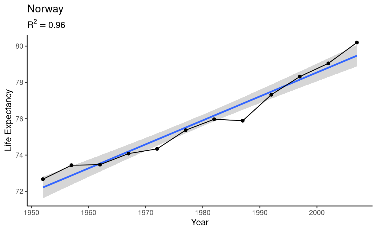
Writing our own functions can be very helpful for making our code more readable. It allows us to separate certain steps of your analysis from the rest, look at them in isolation to test and validate them, and also allows us to give them reasonable names. Let’s look at a couple of examples and get you writing functions! Say we have this idea, where we filter the gapminder dataset for one country, check how linear the relationship between year and life expectancy is and then create a plot.
These three function from the broom package tell us more about our linear model created with lm. It is part of the tidymodels framework.
broom::tidy(model)
# A tibble: 2 x 5
  term        estimate std.error statistic      p.value
  <chr>          <dbl>     <dbl>     <dbl>        <dbl>
1 (Intercept) -185.     16.2         -11.4 0.000000460
2 year 0.132 0.00819 16.1 0.0000000176broom::augment(model)
# A tibble: 12 x 8
   lifeExp  year .fitted  .resid   .hat .sigma .cooksd .std.resid
     <dbl> <dbl>   <dbl>   <dbl>  <dbl>  <dbl>   <dbl>      <dbl>
 1    72.7  1952    72.2  0.455  0.295   0.483 0.256        1.11
 2    73.4  1957    72.9  0.566  0.225   0.470 0.250        1.31
 3    73.5  1962    73.5 -0.0640 0.169   0.516 0.00209     -0.143
 4    74.1  1967    74.2 -0.114  0.127   0.515 0.00450     -0.249
 5    74.3  1972    74.9 -0.513  0.0991  0.484 0.0671      -1.10
 6    75.4  1977    75.5 -0.143  0.0851  0.514 0.00434     -0.306
 7    76.0  1982    76.2 -0.203  0.0851  0.511 0.00872     -0.433
 8    75.9  1987    76.8 -0.943  0.0991  0.396 0.226       -2.03
 9    77.3  1992    77.5 -0.172  0.127   0.512 0.0103      -0.377
10    78.3  1997    78.2  0.168  0.169   0.512 0.0144       0.376
11    79.0  2002    78.8  0.238  0.225   0.508 0.0443       0.553
12 80.2 2007 79.5 0.725 0.295 0.429 0.649 1.76 broom::glance(model)
# A tibble: 1 x 12
  r.squared adj.r.squared sigma statistic   p.value    df logLik   AIC
      <dbl>         <dbl> <dbl>     <dbl>     <dbl> <dbl>  <dbl> <dbl>
1     0.963         0.959 0.490      260.   1.76e-8     1  -7.37  20.7
# … with 4 more variables: BIC <dbl>, deviance <dbl>,
#   df.residual <int>, nobs <int>
The \(R^2\) value tells us, how well a straight line fits to our data. It can assume values between 0 and 1.
model_glance <- broom::glance(model)

text <- substitute(R^2 == rsq,
                   list(rsq = round(model_glance$r.squared, 2)))

filterd_data %>%
  ggplot(aes(year, lifeExp)) +
  geom_smooth(method = "lm") +
  geom_line() +
  geom_point() +
  theme_classic() +
  labs(
    x = "Year",
    y = "Life Expectancy",
    title = "Norway",
    subtitle = text
  )
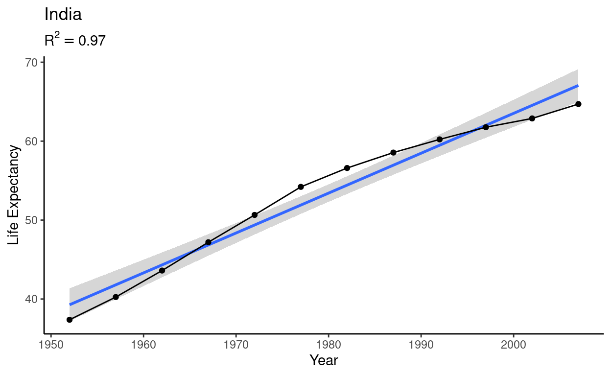
Then we get curious and want to know how this graph looks for another country. So we copy and paste our code and replace the name of the country. And yet again, we want to see this plot for another country, so we copy and paste our code, change the country name and keep going. This is when we remember, that there is an easier way to deal with this repetition. We look at our code again and identify the things that stay the same and the things that change during each copy and pasting. The things that stay the same will be the body of our function, the things that change will be variables in the body that we pass to the function as arguments. In our example, there is only one thing that changes every time: the name of the country. So we build the following function:
plot_life_exp_for_country <- function(country_name) {
  filterd_data <- gapminder %>%
    filter(country == country_name)

  model <- lm(lifeExp ~ year, data = filterd_data)
  model_glance <- broom::glance(model)
  text <- substitute(R^2 == rsq,
                     list(rsq = round(model_glance$r.squared, 2)))

  filterd_data %>%
    ggplot(aes(year, lifeExp)) +
    geom_smooth(method = "lm") +
    geom_line() +
    geom_point() +
    theme_classic() +
    labs(
      x = "Year",
      y = "Life Expectancy",
      title = country_name,
      subtitle = text
    )
}
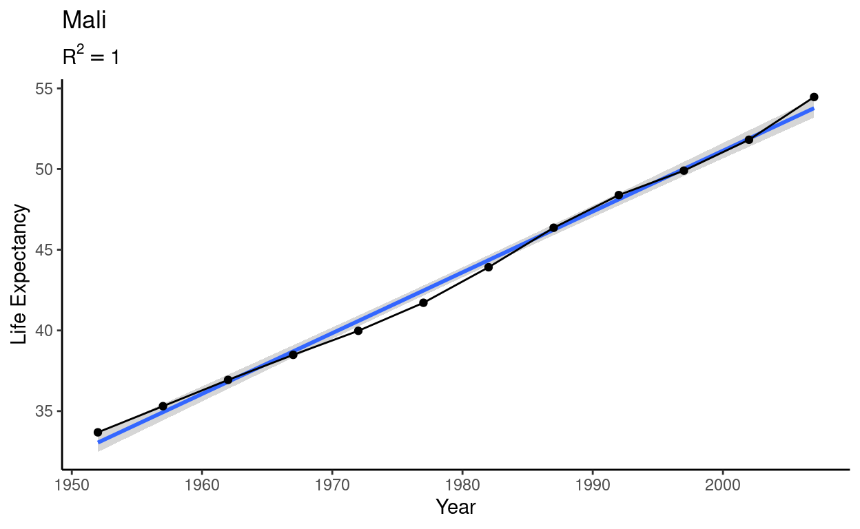
Then we test the function a bunch to make sure it works for different cases:
plot_life_exp_for_country("India")
plot_life_exp_for_country("Mali")
Where to put your Functions
At this point you might wonder where to put this function. A good starting point is to collect your functions near the top of your document or script, below where you load all packages. Another approach, especially if you have functions that you can use for multiple projects, is to put them in a .R file and load this file at the beginning of your document. You can do so using the function source("path/to/file.R"). It runs the R file in your current sessions, so any functions and variables defined in there are now available to you.
source("R/my_funs.R")
Just like this.
say_hello()
[1] "Hello!"I like to store my regular R files (as opposed to Rmd files) in a folder of my project called R. This makes it already look like an R package, in case I decide later on that the functions could be helpful for others as well or I want to share them more easily with colleagues. You can read more about creating your own R packages here (Wickham 2015).
Many Models
Let us use the techniques above to shine light on how life expectancies changed over time. This time, we will utilize the nested data format to store our data alongside models for the data.
nested_gapminder <- gapminder %>%
  nest(-country, -continent) %>%
  mutate(
    model = map(data, ~ lm(lifeExp ~ year, data = .x))
  )

nested_gapminder
# A tibble: 142 x 4
   continent country                  data              model
   <chr>     <chr>                    <list>            <list>
 1 Africa    Algeria                  <tibble [12 × 4]> <lm>
 2 Africa    Angola                   <tibble [12 × 4]> <lm>
 3 Africa    Benin                    <tibble [12 × 4]> <lm>
 4 Africa    Botswana                 <tibble [12 × 4]> <lm>
 5 Africa    Burkina Faso             <tibble [12 × 4]> <lm>
 6 Africa    Burundi                  <tibble [12 × 4]> <lm>
 7 Africa    Cameroon                 <tibble [12 × 4]> <lm>
 8 Africa    Central African Republic <tibble [12 × 4]> <lm>
 9 Africa    Chad                     <tibble [12 × 4]> <lm>
10 Africa    Comoros                  <tibble [12 × 4]> <lm>
# … with 132 more rows
Then, we extract information about the model with some functions form the broom package.
nested_gapminder %>%
  mutate(
    glance = map(model, broom::glance)
  )
# A tibble: 142 x 5
   continent country              data            model glance
   <chr>     <chr>                <list>          <lis> <list>
 1 Africa    Algeria              <tibble [12 × … <lm>  <tibble [1 × …
 2 Africa    Angola               <tibble [12 × … <lm>  <tibble [1 × …
 3 Africa    Benin                <tibble [12 × … <lm>  <tibble [1 × …
 4 Africa    Botswana             <tibble [12 × … <lm>  <tibble [1 × …
 5 Africa    Burkina Faso         <tibble [12 × … <lm>  <tibble [1 × …
 6 Africa    Burundi              <tibble [12 × … <lm>  <tibble [1 × …
 7 Africa    Cameroon             <tibble [12 × … <lm>  <tibble [1 × …
 8 Africa    Central African Rep… <tibble [12 × … <lm>  <tibble [1 × …
 9 Africa    Chad                 <tibble [12 × … <lm>  <tibble [1 × …
10 Africa    Comoros              <tibble [12 × … <lm>  <tibble [1 × …
# … with 132 more rows
Then we go ahead and unnest the information about the model. We can now see, which countries stray the farthest from a straight line by arranging by the \(R^2\) values.
gapminder_modeled <- nested_gapminder %>%
  mutate(
    glance = map(model, broom::glance)
  ) %>%
  unnest(glance) %>%
  arrange(r.squared)

gapminder_modeled
# A tibble: 142 x 16
   continent country     data      model r.squared adj.r.squared sigma
   <chr>     <chr>       <list>    <lis>     <dbl>         <dbl> <dbl>
 1 Africa    Rwanda      <tibble … <lm>     0.0172      -0.0811   6.56
 2 Africa    Botswana    <tibble … <lm>     0.0340      -0.0626   6.11
 3 Africa    Zimbabwe    <tibble … <lm>     0.0562      -0.0381   7.21
 4 Africa    Zambia      <tibble … <lm>     0.0598      -0.0342   4.53
 5 Africa    Swaziland   <tibble … <lm>     0.0682      -0.0250   6.64
 6 Africa    Lesotho     <tibble … <lm>     0.0849      -0.00666  5.93
 7 Africa    Cote d'Ivo… <tibble … <lm>     0.283        0.212    3.93
 8 Africa    South Afri… <tibble … <lm>     0.312        0.244    4.74
 9 Africa    Uganda      <tibble … <lm>     0.342        0.276    3.19
10 Africa    Congo, Dem… <tibble … <lm>     0.348        0.283    2.43
# … with 132 more rows, and 9 more variables: statistic <dbl>,
#   p.value <dbl>, df <dbl>, logLik <dbl>, AIC <dbl>, BIC <dbl>,
#   deviance <dbl>, df.residual <int>, nobs <int>
For a more detailed walk-trough, check out the chapter on “many models” in R for Data Science here (Wickham and Grolemund 2017).
Let’s use this information to build a visualization.
non_linear_countries <- gapminder_modeled %>%
  filter(r.squared < 0.2) %>%
  unnest(data)

non_linear_countries
# A tibble: 72 x 19
continent country year lifeExp pop gdpPercap model r.squared
<chr> <chr> <dbl> <dbl> <dbl> <dbl> <list> <dbl>
1 Africa Rwanda 1952 40 2534927 493. <lm> 0.0172
2 Africa Rwanda 1957 41.5 2822082 540. <lm> 0.0172
3 Africa Rwanda 1962 43 3051242 597. <lm> 0.0172
4 Africa Rwanda 1967 44.1 3451079 511. <lm> 0.0172
5 Africa Rwanda 1972 44.6 3992121 591. <lm> 0.0172
6 Africa Rwanda 1977 45 4657072 670. <lm> 0.0172
7 Africa Rwanda 1982 46.2 5507565 882. <lm> 0.0172
8 Africa Rwanda 1987 44.0 6349365 848. <lm> 0.0172
9 Africa Rwanda 1992 23.6 7290203 737. <lm> 0.0172
10 Africa Rwanda 1997 36.1 7212583 590. <lm> 0.0172
# … with 62 more rows, and 11 more variables: adj.r.squared <dbl>,
# sigma <dbl>, statistic <dbl>, p.value <dbl>, df <dbl>,
# logLik <dbl>, AIC <dbl>, BIC <dbl>, deviance <dbl>,
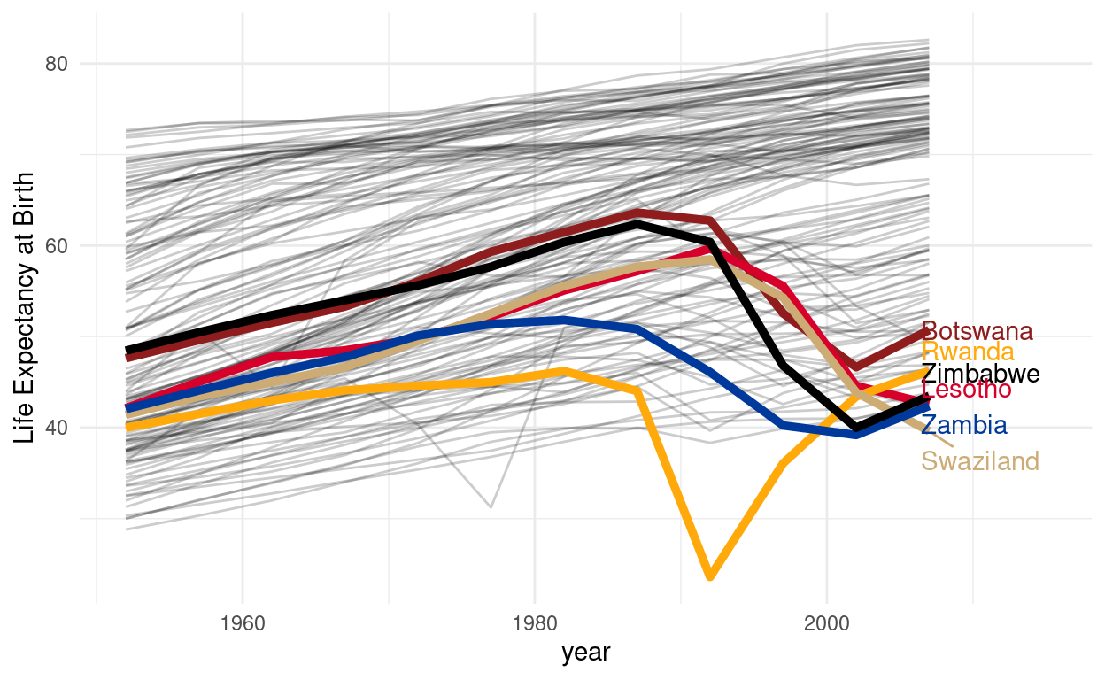
# df.residual <int>, nobs <int>I also like to use this opportunity to mention a couple of packages to take your visualizations the the next level. Today, these are ggrepel to produce labels that dodge each other, and the fisualize package, which contains color scales of tropical fish.
plt <- gapminder %>%
  ggplot(aes(year, lifeExp, group = country)) +
  geom_line(alpha = 0.2) +
  geom_line(data = non_linear_countries,
            mapping = aes(color = country),
            size = 1.7) +
  fishualize::scale_color_fish_d() +
  labs(y = "Life Expectancy at Birth") +
  ggrepel::geom_text_repel(data = filter(non_linear_countries, year == max(year)),
            aes(label = country, color = country),
            hjust = 0, direction = "y") +
  expand_limits(x = 2015) +
  theme_minimal() +
  guides(color = "none")

plt
Sometimes it is also very handy (and probably impressive to whoever receives your report) to turn a plot into an interactive graphic. plotly is a library that produces interactive plots, but we don’t even have to learn about its intricacies because it comes with a function to convert a ggplot to the interactive format that works quite well for a range (but not all) of use-cases:
plotly::ggplotly(plt)
The downward slope of our highlighted countries starting in the 1990s is a result of the ravaging AIDS pandemic. The prominent dips in two of the curves, orange for Rwanda and Cambodia in gray, are the direct consequences of genocides. These dire realities can in no way be summarized in just a couple of colorful lines. I am also in no way qualified to lecture on these topics. A good friend of mine, Timothy Williams, however is a researcher and teacher in the field of conflict and violence with a focus on genocides. He did field work in Cambodia and Rwanda and his book “The Complexity of Evil. Perpetration and Genocide” will be published here on December 18 (Williams, n.d.).
Advanced dplyr
Last but not least, I want to mention a powerful advanced function in dplyr to make your data transformations even more efficient. It is the across function, which we can use inside of dplyr verbs such as mutate and summarise to use one or multiple functions on multiple columns. Let’s look at an example, again with the gapminder dataset. Now, this is sort of a silly example, but let’s say we want the continents and countries in UPPERCASE. We could do:
gapminder %>%
  mutate(
    continent = str_to_upper(continent),
    country = str_to_upper(country)
  )
# A tibble: 1,704 x 6
   continent country  year lifeExp      pop gdpPercap
   <chr>     <chr>   <dbl>   <dbl>    <dbl>     <dbl>
 1 AFRICA    ALGERIA  1952    43.1  9279525     2449.
 2 AFRICA    ALGERIA  1957    45.7 10270856     3014.
 3 AFRICA    ALGERIA  1962    48.3 11000948     2551.
 4 AFRICA    ALGERIA  1967    51.4 12760499     3247.
 5 AFRICA    ALGERIA  1972    54.5 14760787     4183.
 6 AFRICA    ALGERIA  1977    58.0 17152804     4910.
 7 AFRICA    ALGERIA  1982    61.4 20033753     5745.
 8 AFRICA    ALGERIA  1987    65.8 23254956     5681.
 9 AFRICA    ALGERIA  1992    67.7 26298373     5023.
10 AFRICA    ALGERIA  1997    69.2 29072015     4797.
# … with 1,694 more rows
And now everyone is really shouty. But we had some repetition in our code. Wouldn’t it be cool, to just say: “Apply the function str_to_upper to these columns.”
gapminder %>%
  mutate(
    across(c(continent, country), str_to_upper)
  )
# A tibble: 1,704 x 6
   continent country  year lifeExp      pop gdpPercap
   <chr>     <chr>   <dbl>   <dbl>    <dbl>     <dbl>
 1 AFRICA    ALGERIA  1952    43.1  9279525     2449.
 2 AFRICA    ALGERIA  1957    45.7 10270856     3014.
 3 AFRICA    ALGERIA  1962    48.3 11000948     2551.
 4 AFRICA    ALGERIA  1967    51.4 12760499     3247.
 5 AFRICA    ALGERIA  1972    54.5 14760787     4183.
 6 AFRICA    ALGERIA  1977    58.0 17152804     4910.
 7 AFRICA    ALGERIA  1982    61.4 20033753     5745.
 8 AFRICA    ALGERIA  1987    65.8 23254956     5681.
 9 AFRICA    ALGERIA  1992    67.7 26298373     5023.
10 AFRICA    ALGERIA  1997    69.2 29072015     4797.
# … with 1,694 more rows
Not that is raw power! We can be even more general and ask R to apply the function to all columns that contain text:
gapminder %>%
  mutate(
    across(where(is.character), str_to_upper)
  )
# A tibble: 1,704 x 6
   continent country  year lifeExp      pop gdpPercap
   <chr>     <chr>   <dbl>   <dbl>    <dbl>     <dbl>
 1 AFRICA    ALGERIA  1952    43.1  9279525     2449.
 2 AFRICA    ALGERIA  1957    45.7 10270856     3014.
 3 AFRICA    ALGERIA  1962    48.3 11000948     2551.
 4 AFRICA    ALGERIA  1967    51.4 12760499     3247.
 5 AFRICA    ALGERIA  1972    54.5 14760787     4183.
 6 AFRICA    ALGERIA  1977    58.0 17152804     4910.
 7 AFRICA    ALGERIA  1982    61.4 20033753     5745.
 8 AFRICA    ALGERIA  1987    65.8 23254956     5681.
 9 AFRICA    ALGERIA  1992    67.7 26298373     5023.
10 AFRICA    ALGERIA  1997    69.2 29072015     4797.
# … with 1,694 more rows
It also works with summarise, for example to create summaries across a range of columns. And we can supply more than one function to calculate using a named list:
gapminder %>%
  summarise(
    across(year:gdpPercap, list(mean = mean, total = sum))
  )
# A tibble: 1 x 8
  year_mean year_total lifeExp_mean lifeExp_total  pop_mean  pop_total
      <dbl>      <dbl>        <dbl>         <dbl>     <dbl>      <dbl>
1     1980.    3373068         59.5       101344. 29601212.    5.04e10
# … with 2 more variables: gdpPercap_mean <dbl>,
#   gdpPercap_total <dbl>
You are on you way to becoming a true data wizard! After today, you should be familiar with:
- importing data into R
- the concept of tidy data
- the grammar of graphics
- the basic dplyr verbs for data wrangling
- a project-based workflow
- writing and using functions
We will then use these foundations to experience statistical concepts ourselves in the next lectures.
Exercises
The whole Deal
I want to get you playing around with data, so keep in mind that the solutions for this exercise are not set in stone. There is often more than one viable way of graphing the same dataset and we will use the Office Hour to talk about the advantages and disadvantages of approaches that you came up with.
Roman emperors
The first exercise uses a dataset about roman emperors from the tidytuesday project (link). You can import it with:
emperors <- readr::read_csv("https://raw.githubusercontent.com/rfordatascience/tidytuesday/master/data/2019/2019-08-13/emperors.csv")
Here are a couple of questions to answer. Decide for yourselves if a particular question is best answered using a visualization, a table or a simple sentence.
- What was the most popular way to rise to power?
- I what are the most common causes of death among roman emperors, what (or who) killed them?
- Which dynasty was the most successful?
- Firstly, how often did each dynasty reign?
- Secondly, how long where the reigns?
- Which dynasty would you rather be a part of, if your goal is to live the longest?
Dairy Products in the US
Another dataset (link) concerns dairy product consumption per person in the US across a number of years. Load it with
dairy <- readr::read_csv("https://raw.githubusercontent.com/rfordatascience/tidytuesday/master/data/2019/2019-01-29/milk_products_facts.csv")
- All masses are given in lbs (pounds), can you convert them to kg?
- Which products lost their customer base over time, which ones won?
Above all, have some fun! If you make interesting findings along the way, go ahead and produce plots to highlight it.
Resources