Lecture 8

… in which we venture into the unknown to show an example data analysis, gather more data with webscraping and build a small app.

In today’s lecture, the script is the result of experimenting with unseen data as seen in the video. You can refer back to it in order to get the code if the video goes to fast. By itself, the script will be less useful than the script for regular lectures. I hope you can learn something from how I approach a new task and how I handle mistakes and errors. The video is largely unedited; I only removed a portion where all attempts at webscraping failed for a while because my internet connection was gone…

Video

Watch today’s video here:

Slides

This special Christmas video has no slides.

Script

library(tidyverse)
library(rvest)
library(glue)

Christmas Theme!

• Christmas RStudio theme: https://github.com/gadenbuie/rsthemes

Advanced Rmarkdown

• Using the RStudio plugin to insert citations directly from Zotero
  • preview of https://blog.rstudio.com/2020/11/09/rstudio-1-4-preview-citations/
• Other output formats:
  • https://bookdown.org/yihui/rmarkdown/
  • https://github.com/rstudio/rticles
    • note: tinytex package for pdf outputs

Finding Help Easier

• https://reprex.tidyverse.org/

Into the Unknown: An Example Analysis of Unseen Data

Into the Unknown, from the giphy api

The Data: Fast Food Entrees

Find the data here.

fastfood <- read_csv("data/fastfood.csv") %>% 
  select(-salad, -X1) %>%  
  distinct(restaurant, item, .keep_all = TRUE)

fastfood

# A tibble: 513 x 16
   restaurant item        calories cal_fat total_fat sat_fat trans_fat
   <chr>      <chr>          <dbl>   <dbl>     <dbl>   <dbl>     <dbl>
 1 Mcdonalds  Artisan Gr…      380      60         7       2       0  
 2 Mcdonalds  Single Bac…      840     410        45      17       1.5
 3 Mcdonalds  Double Bac…     1130     600        67      27       3  
 4 Mcdonalds  Grilled Ba…      750     280        31      10       0.5
 5 Mcdonalds  Crispy Bac…      920     410        45      12       0.5
 6 Mcdonalds  Big Mac          540     250        28      10       1  
 7 Mcdonalds  Cheeseburg…      300     100        12       5       0.5
 8 Mcdonalds  Classic Ch…      510     210        24       4       0  
 9 Mcdonalds  Double Che…      430     190        21      11       1  
10 Mcdonalds  Double Qua…      770     400        45      21       2.5
# … with 503 more rows, and 9 more variables: cholesterol <dbl>,
#   sodium <dbl>, total_carb <dbl>, fiber <dbl>, sugar <dbl>,
#   protein <dbl>, vit_a <dbl>, vit_c <dbl>, calcium <dbl>

Watch the video to find out how these small data cleaning steps came about.

fastfood %>% 
  count(restaurant)

# A tibble: 8 x 2
  restaurant      n
  <chr>       <int>
1 Arbys          55
2 Burger King    70
3 Chick Fil-A    27
4 Dairy Queen    42
5 Mcdonalds      57
6 Sonic          53
7 Subway         96
8 Taco Bell     113

Counting things is always a good sanity check for your data.

fastfood %>% 
  count(restaurant, item, sort = TRUE)

# A tibble: 513 x 3
   restaurant item                                  n
   <chr>      <chr>                             <int>
 1 Arbys      2 piece Prime-Cut Chicken Tenders     1
 2 Arbys      3 piece Prime-Cut Chicken Tenders     1
 3 Arbys      5 piece Prime-Cut Chicken Tenders     1
 4 Arbys      Arby-Q Sandwich                       1
 5 Arbys      Arby's Melt                           1
 6 Arbys      Beef 'n Cheddar Classic               1
 7 Arbys      Beef 'n Cheddar Mid                   1
 8 Arbys      Bourbon BBQ Brisket Sandwich          1
 9 Arbys      Bourbon BBQ Chicken Sandwich          1
10 Arbys      Bourbon BBQ Steak Sandwich            1
# … with 503 more rows

We will need the names of the restaurants.

restaurants <- unique(fastfood$restaurant)
restaurants

[1] "Mcdonalds"   "Chick Fil-A" "Sonic"       "Arbys"      
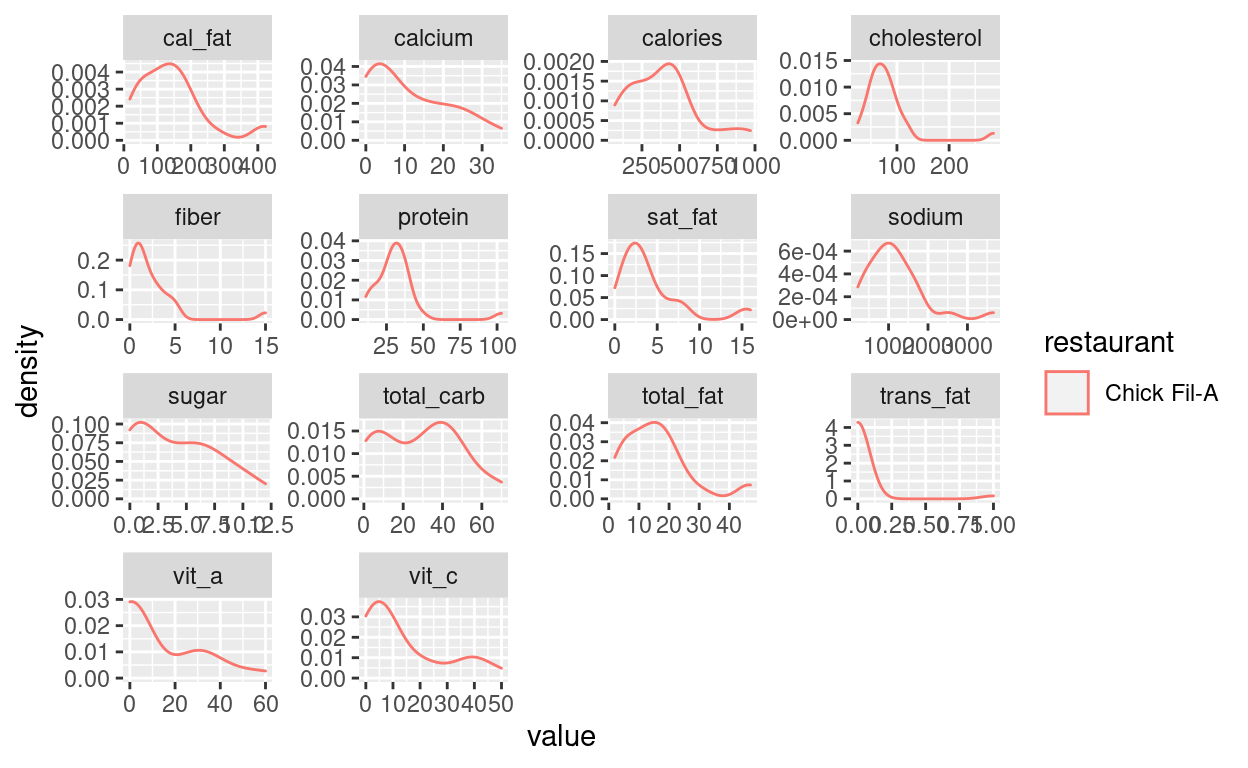
[5] "Burger King" "Dairy Queen" "Subway"      "Taco Bell"  

This is not a very refined plot. I really wanted to get to to the webscraping part to show you new exciting things.

fastfood %>% 
  filter(restaurant == restaurants[2]) %>% 
  pivot_longer(-c(restaurant, item)) %>% 
  ggplot(aes(value, color = restaurant)) +
  geom_density() +
  facet_wrap(~ name, scales = "free")

Webscraping with rvest

• https://rvest.tidyverse.org/

The restaurant names on the links to the complaints-website are slightly different to the names we have in our fastfood dataset. Some things are just faster to do manually than figuring out an algorithmic way of achieving. Although in this case, it could have been easier because there is only one exception (sonic) to “make everything lowercase and replace space with hyphens.”

restaurant_names <- c(
  "mcdonalds",
  "chick-fil-a",
  "sonic-drive-in",
  "arbys",
  "burger-king",
  "dairy-queen",
  "subway",
  "taco-bell"
)

Get some data! Try it on one example, then write a function to do so. Then test the function on some examples.

n <- 1
restaurant <- restaurant_names[8]
url <- glue("https://www.complaintsboard.com/{restaurant}/page/{1}")

get_complaints <- function(url) {
  read_html(url) %>% 
  html_nodes(css = ".list-text") %>% 
  html_text()
}

This chunk is set to eval=FALSE. Meaning we can still run it manually but it will not run every time we knit the document or press “run all chunks.” This enables us to keep the code for a long running computation in the document while not having to run it every time. A more elegant approach would have been to refactor this into it’s own R script after the initial exploration.

complaints <- crossing(
  restaurant = restaurant_names,
  n = 1:30
) %>% 
  mutate(
    url = glue("https://www.complaintsboard.com/{restaurant}/page/{n}"),
    complaints = map(url, possibly(get_complaints, ""))
  )

write_rds(complaints, "data/complaints.rds")

Now we can load the scraped data.

complaints <- read_rds("data/complaints.rds")

The is a lot of steps happening here. First, we use the tidytext package to extract words from the complaints, then we remove very common words called stop words. We then get the most commong words per restaurant and finally match the original restaurant names with the names we had to use for the webscarping links.

names <- tibble(
  restaurants,
  restaurant_names
)

top_complaints <- complaints %>% 
  unnest_longer(complaints) %>% 
  tidytext::unnest_tokens(input = complaints, output = "word", token = "words") %>%
  anti_join(tidytext::stop_words, by = c("word")) %>% 
  count(restaurant, word, sort = TRUE) %>%
  group_by(restaurant) %>% 
  slice_max(order_by = n, n = 15) %>% 
  ungroup() %>% 
  left_join(names, by = c("restaurant" = "restaurant_names")) %>% 
  select(-restaurant) %>% 
  rename(restaurant = restaurants)

top_complaints %>% 
  rmarkdown::paged_table()

Next, we do a bunch of copy-pasting to quickly prototype an app, where the user can select a restaurant, get a quick overview of the feature distributions and see the most common words in complaints.

A shiny app

https://shiny.rstudio.com/

See app.R in the folder for lecture 8. Note, that because shiny apps are usually in their own project, not in some nested file structure of a course website, there are some shenanigans going on with the file paths. When run locally, R still has the working directory of the project. But when deployed, only the folder in which the app.R file lives is deployed, with no notion of being at the end of some project file path. So the folder where the app.R file lives becomes the new file path when the app is deployed online.

Feedback

I will send round a link with a feedback form. It is anonymous, so I have no way of tracking who submitted it. I will just assume you all did and count it as a completed exercise.