Introduction to Data Analysis with R: Lecture 2

Jannik Buhr

Video

Slides

Script

Note:
I try to be vocal about what the code does in plain English while I type it and learning the “translations” of symbols and keywords can help you, too. After a while, programming can feel a lot more like having a conversation with your digital assistant or a helpful friend. The boundary between human languages and computer languages is more blurry than you might think.

Before we get deeper into R, let’s talk a little bit about our Home when working with R: RStudio.

Making Ourselves at Home in RStudio

Important Settings

I highlighted 3 settings that I consider important to change from their default values. The first two might seem odd at first glance.

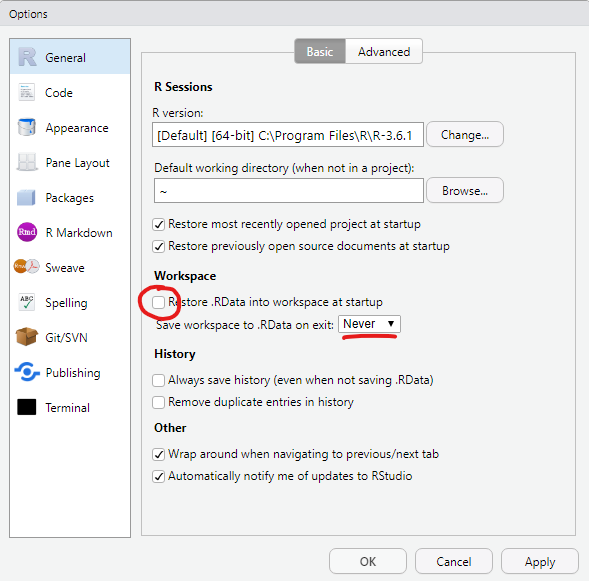
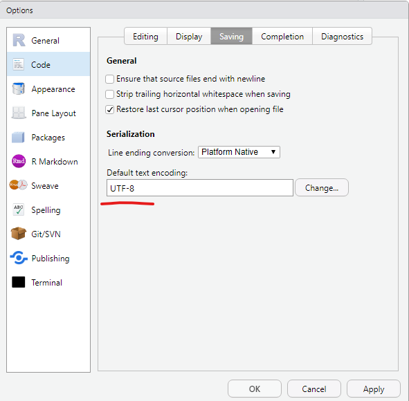
The workspace that RStudio would save as .RData contains all objects created in a session, which is, what we can see in the Environment pane (by default in the top right panel, bottom right in my setup). Why would we not want to load the objects we created in the last session into our current session automatically? The reason is reproducibility. We want to make sure that everything our analysis needs is in the script. It creates our variables and plots from the raw data and should be the sole source of truth. Given the raw data and the script, everyone should be able to reproduce our results. The third setting (text encoding) is also concerned with collaboration. It makes sure that our text files and special characters in them (like German umlauts) look the same on different operating systems like Windows, iOS and Linux.

A Project-based Workflow

Last week we simply went ahead and created a script file and an Rmarkdown file in some folder on our computer. But how does R known, where the script is? How does it know, where to look, when we tell it to read in a file or save a plot? The main folder where R starts is called the working directory. To find out, what our current working directory is, we execute the function getwd() for get working directory:

getwd()

[1] "/home/jannik/Documents/projects/teaching/dataIntro20/_lectures/lecture2"

This will look slightly different depending on you operating system. The next function I want you to know, but never use:

setwd("some/file/path")

“Why should I not use it?” you might ask. Let’s assume I use the function to set the working directory as seen above:

setwd("/home/jannik/Documents/projects/teaching/dataIntro20/_lectures/lecture2")

Now, when I give the file to you to test my analysis, chances are very low that it would work. Because you are likely not called Jannik and even more likely don’t have the same folder structure that I had.

So what we want instead of these absolute file paths, is a relative file paths that start in the folder that our scripts are in. This is what RStudio Projects are for. It is basically just a folder with a special file that ends in .Rproj, but as soon as R finds this file in the folder, the working directory will automatically be this folder. So when you share this folder, it will still just work.

Go ahead and use the blue R button in the top right corner to create a New Project. I recommend you do this either as one project for the whole course or with one project per week. Projects are also convenient because they save what files you had open and so forth.

There is one thing I didn’t tell you about Rmarkdown documents, yet. Their working directory is always the folder they are in, even if they are in some subdirectory of a project. In a way this also means that you don’t necessarily need a project to work with Rmarkdown, but having one anyway makes it easier to keep track of your files and have a consistent structure.

Working in Style

Now that we have a cosy project for today, let’s also make sure we are working in style and are feeling right at home in RStudio. This blogpost provides excellent gifs for the different settings in RStudio and even for Rmarkdown troubleshooting. I am also fond of the rsthemes package for additional appearances.

A Data Analysis Workflow

We are getting close to importing our very first dataset from a file into R. Generally, this is the first thing that needs to happen with any data analysis and we will cover it today. The data I provided is already pretty tidy so we will start with that and build some visualizations. The communicate-part is also covered, because we are working in Rmarkdown after all, which is designed to communicate our findings. Later, we will also have a look at some less tidy data, but not before having defined what “tidy data” is.

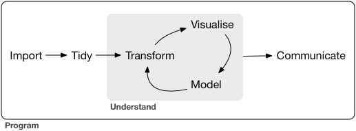
Figure 1: Figure from Wickham and Grolemund (2017).

Reading Data with `readr`

The package responsible for loading data in the tidyverse is called readr, so we start by loading the whole tidyverse.

Note, that in general, we could also load just the readr package with library(readr), but we need the rest of the tidyverse later on anyways. There is also the option to not load a package at all but rather only use one function from a package by prefixing the function with the package name and two colons (::) Like so: readr::read_csv("...").

library(tidyverse)

Without further ado, let’s download the data for today. In fact, there are multiple ways to go about this. We could download the whole course folder from GitHub by following the link in the top right corner of this website and then using the download button:

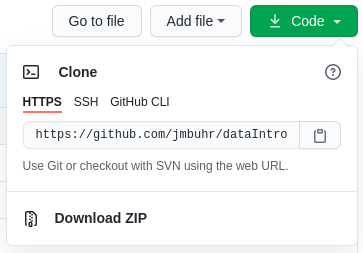
You will then find the data in the folder ./_lectures/lecture2/data/.

Or we can navigate to the file on GitHub. Follow this link: files, click on one of the files and then click on raw:

From there you can copy the link displayed in your browser address field and download the file straight from R:

download.file("https://raw.githubusercontent.com/jmbuhr/dataIntro20/master/_lectures/lecture2/data/gapminder.csv",
              "data/gapminder.csv")

The folder to download your data to (./data) must be created in advance. This is an example for a relative path (an absolute path would start with / or a drive letter like C:).

Now we can finally load in the data and store it in a variable. When working with file paths, RStudio’s autocompletion is especially helpful. We can trigger it with Tab or Ctrl+Space.

gapminder <- read_csv("data/gapminder.csv")

readr will also tell you the datatypes it guessed for the columns. Let’s inspect our dataset:

gapminder

# A tibble: 1,704 x 6
   country     continent  year lifeExp      pop gdpPercap
   <chr>       <chr>     <dbl>   <dbl>    <dbl>     <dbl>
 1 Afghanistan Asia       1952    28.8  8425333      779.
 2 Afghanistan Asia       1957    30.3  9240934      821.
 3 Afghanistan Asia       1962    32.0 10267083      853.
 4 Afghanistan Asia       1967    34.0 11537966      836.
 5 Afghanistan Asia       1972    36.1 13079460      740.
 6 Afghanistan Asia       1977    38.4 14880372      786.
 7 Afghanistan Asia       1982    39.9 12881816      978.
 8 Afghanistan Asia       1987    40.8 13867957      852.
 9 Afghanistan Asia       1992    41.7 16317921      649.
10 Afghanistan Asia       1997    41.8 22227415      635.
# … with 1,694 more rows

The gapminder dataset (Bryan 2017) is an excerpt from the gapminder project and contains the life expectancy at birth for 142 countries at 5 year intervals between 1952 and 2007. It also contains the population and the Gross Domestic Product (GDP) per Inhabitant. We will built a visualization later on.

read_csv can even read data from a url straight away, without the need for us to download the file ourselves, but we usually want a copy of the data locally. For the curious run this:

read_csv("https://raw.githubusercontent.com/jmbuhr/dataIntro20/master/_lectures/lecture2/data/gapminder.csv")

So, this all went smoothly. But this will not always be the case. We will now look at common hurdles when importing data

Common Hurdles when Importing Data

The function we just used was called read_csv, because it reads a file format that consists of comma separated values. Look at the raw file in a text editor (not word) like notepad or RStudio to see why. But the file extension .csv can sometimes be lying…

Because in German, the comma is used to separate decimal numbers (vs. the dot in English), a lot of Software will output a different type of csv-file when configured in German. It will still call it csv, but actually it is separated by semicolons! We have a special function for this:

read_csv2("data/gapminder_csv2.csv")

When looking through the autocompletion options that pop up when you are typing the function name, you might have noticed a similar function read.csv and read.csv2. These are the functions that come with R, without any packages like the tidyverse. You can of course use those as well, but the tidyverse functions provide a more consistent experience and have less surprising quirks. I am teaching the tidyverse first, because it allows you to do more while having to learn less edge cases.

If we look at yet another file data/gapminder_tsv.txt, we notice that the file extension doesn’t tell us much about the format, only that it is text (as opposed to a binary format only computers can read). If we look into the file:

read_lines("data/gapminder_tsv.txt", n_max = 3)

[1] "country\tcontinent\tyear\tlifeExp\tpop\tgdpPercap"    
[2] "Afghanistan\tAsia\t1952\t28.801\t8425333\t779.4453145"
[3] "Afghanistan\tAsia\t1957\t30.332\t9240934\t820.8530296"

We notice that the values are separated by ", a special sequence that stands for the tab character. The read_tsv function will do the job.

If the separator (also called delimiter) is even more obscure, we can use the general function read_delim. Say a co-worker misunderstood us and thought tsv stands for “Tilde separated values,” we can still read his file.

read_lines("data/obscure_file.tsv", n_max = 3)

[1] "country~continent~year~lifeExp~pop~gdpPercap"    
[2] "Afghanistan~Asia~1952~28.801~8425333~779.4453145"
[3] "Afghanistan~Asia~1957~30.332~9240934~820.8530296"

read_delim("data/obscure_file.tsv", delim = "~")

There are more ways in which raw data can be messy or hard to read depending on the machine but I can’t show all of them. One common thing you will encounter though is measurement machines writing some additional information in the first couple of lines before the actual data (like the time of the measurement). In this example:

read_lines("data/gapminder_messier.csv", n_max = 4)

[1] "# Some comment about the data"                   
[2] "And maybe a personal note"                       
[3] "country,continent,year,lifeExp,pop,gdpPercap"    
[4] "Afghanistan,Asia,1952,28.801,8425333,779.4453145"

The first 2 lines are not part of the data. Reading the file normally as a csv would produce something weird: Because the first line does not contain any commata, it will assume that the file contains only one column and also report a bunch of parsing failures. Parsing is the act of turning data represented as raw text into a useful format, like a table of numbers.

read_csv("data/gapminder_messier.csv", n_max = 3)

# A tibble: 3 x 1
  `# Some comment about the data`
  <chr>                          
1 And maybe a personal note      
2 country                        
3 Afghanistan

We can fix this by telling R to skip the first 2 lines entirely:

read_csv("data/gapminder_messier.csv", skip = 2, n_max = 3)

# A tibble: 3 x 6
  country     continent  year lifeExp      pop gdpPercap
  <chr>       <chr>     <dbl>   <dbl>    <dbl>     <dbl>
1 Afghanistan Asia       1952    28.8  8425333      779.
2 Afghanistan Asia       1957    30.3  9240934      821.
3 Afghanistan Asia       1962    32.0 10267083      853.

I was using the n_max argument of the functions above to save space in this lecture script.

In the video I forgot to mention that I also included an excel file to practice. We can read it using a function from the readxl package. This package is automatically installed with the tidyverse, but it is not loaded along with the other packages via library(tidyverse). We can either load it with library(readxl) or refer to a single function from the package without loading the whole thing using double colons (::):

readxl::read_xlsx("./data/gapminder.xlsx")

Now, that we learned about some of the ways in which raw data can be structured, let us go back to the original data that we read in and saved in the variable gapminder.

country	continent	year	lifeExp	pop	gdpPercap
Afghanistan	Asia	1952	28.801	8425333	779.4453
Afghanistan	Asia	1957	30.332	9240934	820.8530
Afghanistan	Asia	1962	31.997	10267083	853.1007
Afghanistan	Asia	1967	34.020	11537966	836.1971
Afghanistan	Asia	1972	36.088	13079460	739.9811
Afghanistan	Asia	1977	38.438	14880372	786.1134

Wrangling Data with `dplyr`

There a are a number of ways in which we can manipulate data. Of course I mean manipulate in it’s original sense, not the malicious one. This is sometimes referred to as data wrangling and within the tidyverse, this is a job for the dplyr package (short for data plyer, the tool you see in the logo).

dplyr provides functions for various operations on our data. Theses functions are sometimes also called dplyr verbs. All of them take a tibble or data.frame as input (plus additional parameters) and always return a tibble.

Figure 2: (“Artwork by @Allison_horst” 2020)

select

The first verb we introduce is used to select columns. And hence, it is called select. The first argument is always the data, followed by an arbitrary number of column names. We can recognize functions the take an arbitrary number of additional arguments by the ... in the autocompletion and help page.

select(gapminder, country, year, pop)

# A tibble: 1,704 x 3
   country      year      pop
   <chr>       <dbl>    <dbl>
 1 Afghanistan  1952  8425333
 2 Afghanistan  1957  9240934
 3 Afghanistan  1962 10267083
 4 Afghanistan  1967 11537966
 5 Afghanistan  1972 13079460
 6 Afghanistan  1977 14880372
 7 Afghanistan  1982 12881816
 8 Afghanistan  1987 13867957
 9 Afghanistan  1992 16317921
10 Afghanistan  1997 22227415
# … with 1,694 more rows

It might be confusing why we don’t need quotation marks around the column names like we do when we select and element from a vector by name as in:

c(first = 1, second = 2)["first"]

first 
    1

This concept is known as quasiquotation or data masking. It is quite unique to R, but it allows functions to known about the content of the data that is passed to them and use this as the environment in which they do their computations and search for variable names. So while the variable country doesn’t exist in the global environment, it does exist as a column of the gapminder tibble. dplyr functions always look in the data first when they search for names.

The help page for select tells us more about the different ways in which we can select columns. Here are a couple of examples without the output, rum them in your R session to confirm that they do what you think they do. (but do have a look at the help pages yourselves, they are quite well written).

select(gapminder, where(is.numeric))
select(gapminder, country:lifeExp)
select(gapminder, starts_with("c"))
select(gapminder, c(1, 3, 4))

filter

Figure 3: (“Artwork by @Allison_horst” 2020)

After selecting columns it is only natural to ask how to select rows. This is achieved with the function filter. For example, we can filter for all years smaller than 2000:

filter(gapminder, year < 2000)

# A tibble: 1,420 x 6
   country     continent  year lifeExp      pop gdpPercap
   <chr>       <chr>     <dbl>   <dbl>    <dbl>     <dbl>
 1 Afghanistan Asia       1952    28.8  8425333      779.
 2 Afghanistan Asia       1957    30.3  9240934      821.
 3 Afghanistan Asia       1962    32.0 10267083      853.
 4 Afghanistan Asia       1967    34.0 11537966      836.
 5 Afghanistan Asia       1972    36.1 13079460      740.
 6 Afghanistan Asia       1977    38.4 14880372      786.
 7 Afghanistan Asia       1982    39.9 12881816      978.
 8 Afghanistan Asia       1987    40.8 13867957      852.
 9 Afghanistan Asia       1992    41.7 16317921      649.
10 Afghanistan Asia       1997    41.8 22227415      635.
# … with 1,410 more rows

Or all the rows where the country is “New Zealand”:

filter(gapminder, country == "New Zealand")

# A tibble: 12 x 6
   country     continent  year lifeExp     pop gdpPercap
   <chr>       <chr>     <dbl>   <dbl>   <dbl>     <dbl>
 1 New Zealand Oceania    1952    69.4 1994794    10557.
 2 New Zealand Oceania    1957    70.3 2229407    12247.
 3 New Zealand Oceania    1962    71.2 2488550    13176.
 4 New Zealand Oceania    1967    71.5 2728150    14464.
 5 New Zealand Oceania    1972    71.9 2929100    16046.
 6 New Zealand Oceania    1977    72.2 3164900    16234.
 7 New Zealand Oceania    1982    73.8 3210650    17632.
 8 New Zealand Oceania    1987    74.3 3317166    19007.
 9 New Zealand Oceania    1992    76.3 3437674    18363.
10 New Zealand Oceania    1997    77.6 3676187    21050.
11 New Zealand Oceania    2002    79.1 3908037    23190.
12 New Zealand Oceania    2007    80.2 4115771    25185.

mutate

We are back at manipulating columns, this time by creating new ones or changing old ones. The dplyr verb that does that is called muate. For example, we might want to calculate the total GDP from the GDP per Capita and the population:

mutate(gapminder, gdp = pop * gdpPercap)

# A tibble: 1,704 x 7
   country     continent  year lifeExp      pop gdpPercap          gdp
   <chr>       <chr>     <dbl>   <dbl>    <dbl>     <dbl>        <dbl>
 1 Afghanistan Asia       1952    28.8  8425333      779.  6567086330.
 2 Afghanistan Asia       1957    30.3  9240934      821.  7585448670.
 3 Afghanistan Asia       1962    32.0 10267083      853.  8758855797.
 4 Afghanistan Asia       1967    34.0 11537966      836.  9648014150.
 5 Afghanistan Asia       1972    36.1 13079460      740.  9678553274.
 6 Afghanistan Asia       1977    38.4 14880372      786. 11697659231.
 7 Afghanistan Asia       1982    39.9 12881816      978. 12598563401.
 8 Afghanistan Asia       1987    40.8 13867957      852. 11820990309.
 9 Afghanistan Asia       1992    41.7 16317921      649. 10595901589.
10 Afghanistan Asia       1997    41.8 22227415      635. 14121995875.
# … with 1,694 more rows

Notice, that none of the functions changed the original variable gapminder. They only take an input and return and output, which makes it easier to reason about our code and later chain pieces of code together. How do you change it then? Use the Force! … ahem, I mean, the assignment operator (<-).

gapminder <- mutate(gapminder, gdp = pop * gdpPercap)

Here, the power of dplyr shines. It knows that pop and gdpPercap are columns of the tibble and that gdp refers to the new name of the freshly created column.

Interlude: Begind the magic, handling data with base-R

This section is meant to show you what happens behind the scenes. It is not strictly necessary to understand all the details of it in order to work effectively with the tidyverse, but it helps especially when things don’t go as planned.

So let’s look into handling data with base-R. Last week we briefly covered subsetting of vectors by their indices, their names, or a logical vector:

x <- c(42, 1, 13, 29)
names(x) <- c("first", "second", "third", "fourth")
x

 first second  third fourth 
    42      1     13     29

x[c(1,3)]

first third 
   42    13

x[c("first", "second")]

 first second 
    42      1

x[c(TRUE, FALSE, FALSE, TRUE)]

 first fourth 
    42     29

This subsetting with a logical vector can be used to filter the vector:

select_this <- x < 20
select_this

 first second  third fourth 
 FALSE   TRUE   TRUE  FALSE

x[select_this]

second  third 
     1     13

With data in 2 dimensions, rows and columns, subsetting works similarly. Let’s use the function tibble to create a tibble from vectors:

my_data <- tibble(
  x = c(42, 1, 13, 29),
  y = c(1, 2, 3, 4),
  z = c("z1", "z2", "z3", "z4")
)
my_data

# A tibble: 4 x 3
      x     y z    
  <dbl> <dbl> <chr>
1    42     1 z1   
2     1     2 z2   
3    13     3 z3   
4    29     4 z4

Note:
R is not whitespace sensitive (like python). That means indentation doesn’t change the meaning of the code. We can use this to format our code to look pretty, which is why I started a new line after the opening bracket of tibble(.

Subsetting a tibble like a vector selects columns:

my_data[c(1, 3)]

# A tibble: 4 x 2
      x z    
  <dbl> <chr>
1    42 z1   
2     1 z2   
3    13 z3   
4    29 z4

But if you pass two arguments to the square brackets, separated by commata, we can filter rows and select columns Here, we get the first row in the second and third columns:

my_data[1, c(2, 3)]

# A tibble: 1 x 2
      y z    
  <dbl> <chr>
1     1 z1

If we follow the logic above, we can also filter the data. The comma without any argument afterwards selects all columns.

my_data[my_data$x < 20, ]

# A tibble: 2 x 3
      x     y z    
  <dbl> <dbl> <chr>
1     1     2 z2   
2    13     3 z3

At first glance, the tidyverse way of doing the same is only a little bit shorter. But apart from the fact that we don’t have to repeat the name of the data object my_data (because filter knows where to look for x, whereas [] doesn’t), there is another advantage.

filter(my_data, x < 20)

# A tibble: 2 x 3
      x     y z    
  <dbl> <dbl> <chr>
1     1     2 z2   
2    13     3 z3

The pipe `%>%`

The tidyverse functions are easier to compose (i.e. chain together). To facilitate this, we introduce another operator, a bit like + for numbers or the + to add ggplot components, but specially for functions. The pipe, which you can either type or insert in RStudio with Ctrl+Shift+M, takes it’s left side and passes it as the first argument to the function on the right side:

my_data %>% select(x, z)

# A tibble: 4 x 2
      x z    
  <dbl> <chr>
1    42 z1   
2     1 z2   
3    13 z3   
4    29 z4

And because all main tidyverse functions take data as their first argument, we can chain them together fluently. Additionally, it enables autocompletion of column names inside of the function that gets the data. So back to the gapminder example:

gapminder %>% 
  filter(year > 2000) %>% 
  mutate(gdp = pop * gdpPercap) %>% 
  select(country, year, gdp)

# A tibble: 284 x 3
   country      year           gdp
   <chr>       <dbl>         <dbl>
 1 Afghanistan  2002  18363410424.
 2 Afghanistan  2007  31079291949.
 3 Albania      2002  16153932130.
 4 Albania      2007  21376411360.
 5 Algeria      2002 165447670333.
 6 Algeria      2007 207444851958.
 7 Angola       2002  30134833901.
 8 Angola       2007  59583895818.
 9 Argentina    2002 337223430800.
10 Argentina    2007 515033625357.
# … with 274 more rows

It also reads much nicer in your head, which makes reasoning about the code easier. Without telling you what the above code did, you can understand it, because it reads like English. You can often pronounce the pipe as “and then” in your head, or out-loud, I’m not judging.

Note:
The base-R and the tidyverse way are not mutually exclusive. Sometimes you can mix and match.

arrange

A simple thing you might want from a table is to sort it based on some column. This is what arrange does:

gapminder %>% 
  arrange(year)

# A tibble: 1,704 x 7
   country     continent  year lifeExp      pop gdpPercap          gdp
   <chr>       <chr>     <dbl>   <dbl>    <dbl>     <dbl>        <dbl>
 1 Afghanistan Asia       1952    28.8  8425333      779.      6.57e 9
 2 Albania     Europe     1952    55.2  1282697     1601.      2.05e 9
 3 Algeria     Africa     1952    43.1  9279525     2449.      2.27e10
 4 Angola      Africa     1952    30.0  4232095     3521.      1.49e10
 5 Argentina   Americas   1952    62.5 17876956     5911.      1.06e11
 6 Australia   Oceania    1952    69.1  8691212    10040.      8.73e10
 7 Austria     Europe     1952    66.8  6927772     6137.      4.25e10
 8 Bahrain     Asia       1952    50.9   120447     9867.      1.19e 9
 9 Bangladesh  Asia       1952    37.5 46886859      684.      3.21e10
10 Belgium     Europe     1952    68    8730405     8343.      7.28e10
# … with 1,694 more rows

The helper function desc marks a column to be arranged in descending order. We can arrange by multiple columns, where the first will be most important.

gapminder %>% 
  arrange(desc(year), pop) %>% 
  select(country, year, pop) %>% 
  rename(population = pop)

# A tibble: 1,704 x 3
   country                year population
   <chr>                 <dbl>      <dbl>
 1 Sao Tome and Principe  2007     199579
 2 Iceland                2007     301931
 3 Djibouti               2007     496374
 4 Equatorial Guinea      2007     551201
 5 Montenegro             2007     684736
 6 Bahrain                2007     708573
 7 Comoros                2007     710960
 8 Reunion                2007     798094
 9 Trinidad and Tobago    2007    1056608
10 Swaziland              2007    1133066
# … with 1,694 more rows

I also introduced the rename verb without warning. It does what it says it does, only the order of the names might be confusing. The new name comes first (like when you are creating a new column with mutate). You can also rename within select:

gapminder %>% select(country, year, population = pop)

# A tibble: 1,704 x 3
   country      year population
   <chr>       <dbl>      <dbl>
 1 Afghanistan  1952    8425333
 2 Afghanistan  1957    9240934
 3 Afghanistan  1962   10267083
 4 Afghanistan  1967   11537966
 5 Afghanistan  1972   13079460
 6 Afghanistan  1977   14880372
 7 Afghanistan  1982   12881816
 8 Afghanistan  1987   13867957
 9 Afghanistan  1992   16317921
10 Afghanistan  1997   22227415
# … with 1,694 more rows

summarise

To condense one or multiple columns into summary values, we use summarise: Like with mutate, we can calculate multiple things in one step.

gapminder %>% 
  summarise(
    last_year = max(year),
    average_pop = mean(pop),
    minimal_gdp = min(gdp)
  )

# A tibble: 1 x 3
  last_year average_pop minimal_gdp
      <dbl>       <dbl>       <dbl>
1      2007   29601212.   52784691.

But condensing whole columns into one value, flattening the tibble in the style of Super Mario jumping on mushrooms, is often not what we need. We would rather know the summaries within certain groups. For example the maximal gdp per country. This is what group_by is for.

group_by

group_by is considered an adverb, because it doesn’t change the data itself but it changes how subsequent functions handle the data. For example, if a tibble has groups, all summaries are calculated within these groups:

gapminder %>% 
  group_by(country)

# A tibble: 1,704 x 7
# Groups:   country [142]
   country     continent  year lifeExp      pop gdpPercap          gdp
   <chr>       <chr>     <dbl>   <dbl>    <dbl>     <dbl>        <dbl>
 1 Afghanistan Asia       1952    28.8  8425333      779.  6567086330.
 2 Afghanistan Asia       1957    30.3  9240934      821.  7585448670.
 3 Afghanistan Asia       1962    32.0 10267083      853.  8758855797.
 4 Afghanistan Asia       1967    34.0 11537966      836.  9648014150.
 5 Afghanistan Asia       1972    36.1 13079460      740.  9678553274.
 6 Afghanistan Asia       1977    38.4 14880372      786. 11697659231.
 7 Afghanistan Asia       1982    39.9 12881816      978. 12598563401.
 8 Afghanistan Asia       1987    40.8 13867957      852. 11820990309.
 9 Afghanistan Asia       1992    41.7 16317921      649. 10595901589.
10 Afghanistan Asia       1997    41.8 22227415      635. 14121995875.
# … with 1,694 more rows

For example, let’s look at the range of the life expectancy for each country:

gapminder %>% 
  group_by(country) %>% 
  summarise(lower_life_exp = min(lifeExp),
            upper_life_exp = max(lifeExp))

# A tibble: 142 x 3
   country     lower_life_exp upper_life_exp
   <chr>                <dbl>          <dbl>
 1 Afghanistan           28.8           43.8
 2 Albania               55.2           76.4
 3 Algeria               43.1           72.3
 4 Angola                30.0           42.7
 5 Argentina             62.5           75.3
 6 Australia             69.1           81.2
 7 Austria               66.8           79.8
 8 Bahrain               50.9           75.6
 9 Bangladesh            37.5           64.1
10 Belgium               68             79.4
# … with 132 more rows

summarize removes one level of grouping. If the data was grouped by multiple features, this means that some groups remain. We can make sure that the data is no longer grouped with ungroup.

gapminder %>% 
  group_by(continent, year) %>% 
  summarise(mean_gdpPercap = mean(gdpPercap)) %>% 
  ungroup()

# A tibble: 60 x 3
   continent  year mean_gdpPercap
   <chr>     <dbl>          <dbl>
 1 Africa     1952          1253.
 2 Africa     1957          1385.
 3 Africa     1962          1598.
 4 Africa     1967          2050.
 5 Africa     1972          2340.
 6 Africa     1977          2586.
 7 Africa     1982          2482.
 8 Africa     1987          2283.
 9 Africa     1992          2282.
10 Africa     1997          2379.
# … with 50 more rows

Groups also work within mutate and filter. For example, we can get all rows where the gdp per Person was highest per country:

gapminder %>%
  group_by(country) %>% 
  filter(gdpPercap == max(gdpPercap))

# A tibble: 142 x 7
# Groups:   country [142]
   country     continent  year lifeExp      pop gdpPercap          gdp
   <chr>       <chr>     <dbl>   <dbl>    <dbl>     <dbl>        <dbl>
 1 Afghanistan Asia       1982    39.9   1.29e7      978.      1.26e10
 2 Albania     Europe     2007    76.4   3.60e6     5937.      2.14e10
 3 Algeria     Africa     2007    72.3   3.33e7     6223.      2.07e11
 4 Angola      Africa     1967    36.0   5.25e6     5523.      2.90e10
 5 Argentina   Americas   2007    75.3   4.03e7    12779.      5.15e11
 6 Australia   Oceania    2007    81.2   2.04e7    34435.      7.04e11
 7 Austria     Europe     2007    79.8   8.20e6    36126.      2.96e11
 8 Bahrain     Asia       2007    75.6   7.09e5    29796.      2.11e10
 9 Bangladesh  Asia       2007    64.1   1.50e8     1391.      2.09e11
10 Belgium     Europe     2007    79.4   1.04e7    33693.      3.50e11
# … with 132 more rows

Or we can use groups in mutate to find out, what percentage of it’s continent a country’s population makes up per year:

gapminder %>% 
  group_by(continent, year) %>% 
  mutate(pctPop = pop / sum(pop) * 100)

# A tibble: 1,704 x 8
# Groups:   continent, year [60]
   country   continent  year lifeExp     pop gdpPercap      gdp pctPop
   <chr>     <chr>     <dbl>   <dbl>   <dbl>     <dbl>    <dbl>  <dbl>
 1 Afghanis… Asia       1952    28.8  8.43e6      779.  6.57e 9  0.604
 2 Afghanis… Asia       1957    30.3  9.24e6      821.  7.59e 9  0.591
 3 Afghanis… Asia       1962    32.0  1.03e7      853.  8.76e 9  0.605
 4 Afghanis… Asia       1967    34.0  1.15e7      836.  9.65e 9  0.605
 5 Afghanis… Asia       1972    36.1  1.31e7      740.  9.68e 9  0.608
 6 Afghanis… Asia       1977    38.4  1.49e7      786.  1.17e10  0.624
 7 Afghanis… Asia       1982    39.9  1.29e7      978.  1.26e10  0.494
 8 Afghanis… Asia       1987    40.8  1.39e7      852.  1.18e10  0.483
 9 Afghanis… Asia       1992    41.7  1.63e7      649.  1.06e10  0.521
10 Afghanis… Asia       1997    41.8  2.22e7      635.  1.41e10  0.657
# … with 1,694 more rows

Sometimes you want to refer to the size of the current group inside of mutate or summarise. The function to to just that is called n(). For example, I wonder how many rows of data we have per year.

gapminder %>% 
  group_by(year) %>% 
  summarise(n = n())

# A tibble: 12 x 2
    year     n
   <dbl> <int>
 1  1952   142
 2  1957   142
 3  1962   142
 4  1967   142
 5  1972   142
 6  1977   142
 7  1982   142
 8  1987   142
 9  1992   142
10  1997   142
11  2002   142
12  2007   142

A shortcut for group_by and summarise with n() is the count function:

gapminder %>% 
  count(year)

# A tibble: 12 x 2
    year     n
   <dbl> <int>
 1  1952   142
 2  1957   142
 3  1962   142
 4  1967   142
 5  1972   142
 6  1977   142
 7  1982   142
 8  1987   142
 9  1992   142
10  1997   142
11  2002   142
12  2007   142

In general, you might find after solving a particular problem in a couple of steps that there is a more elegant solution. Do not be discouraged by that! It simply means that there is always more to learn, but the tools you already know by now will get you a very long way and set you on the right track.

I think we learned enough dplyr verbs for now. We can treat ourselves to a little ggplot visualization.

Visualization and our First Encounter with `factor`s

gapminder %>% 
  ggplot(aes(year, lifeExp, group = country)) +
  geom_line(alpha = 0.3) +
  facet_wrap(~ continent)

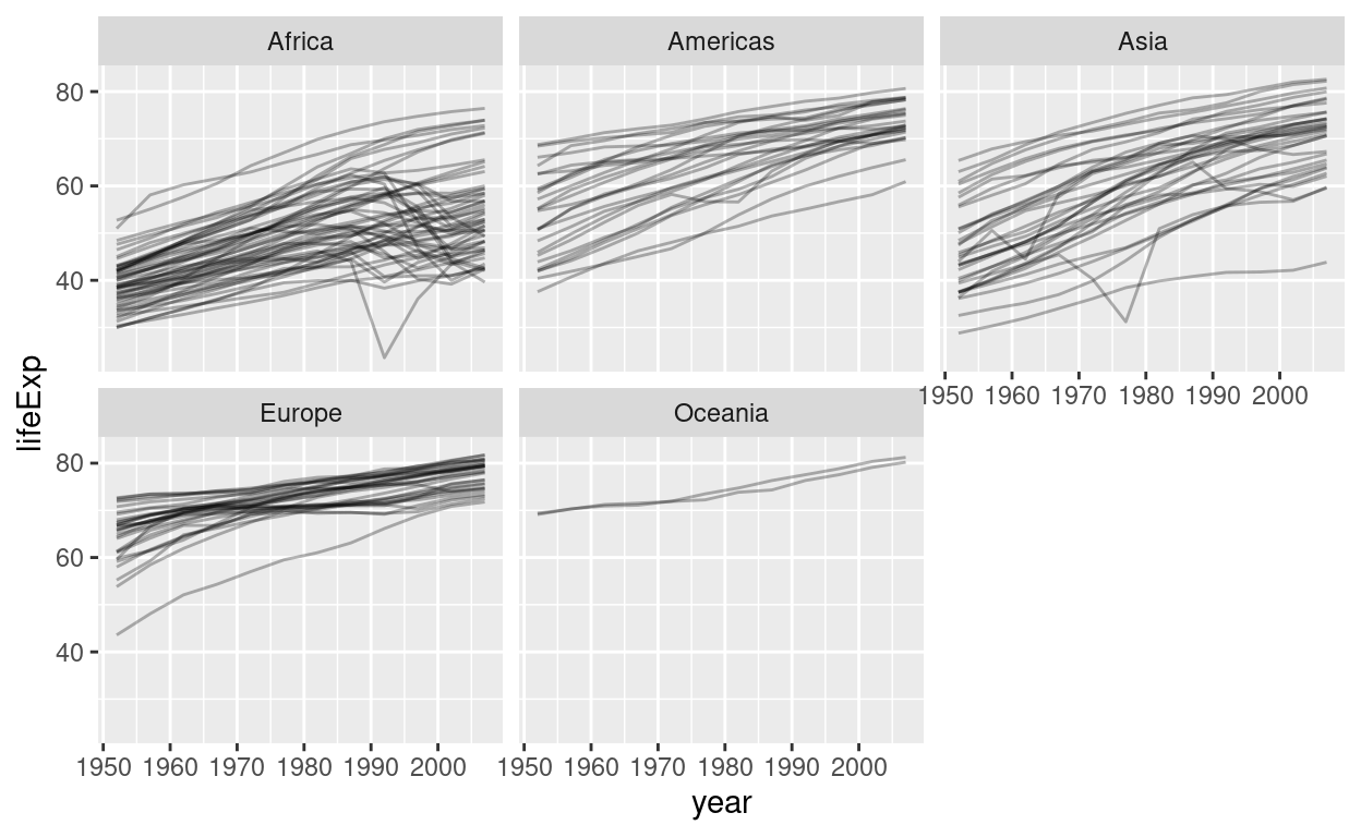
The facet_wrap function slices our plot into theses subplots, a style of plot sometimes referred to as small multiples. At this point you might wonder: “How do I control the order of these facets?” The answer is: With a factor! Any time we have a vector that can be thought of as representing discrete categories (ordered or unordered), we can express this by turning the vector into a factor with the factor function. This enables R’s functions to handle them appropriately. Let’s create a little example. We start out with a character vector.

animals <- c("cat", "dog", "parrot", "whale shark", "bear")
animals

[1] "cat"         "dog"         "parrot"      "whale shark"
[5] "bear"

animals <- factor(animals)
animals

[1] cat         dog         parrot      whale shark bear       
Levels: bear cat dog parrot whale shark

Note the new information R gives us, the Levels, which is all possible values we can put into the factor. They are automatically ordered alphabetically on creation. We can also pass a vector of levels on creation.

animals <- c("cat", "dog", "parrot", "whale shark", "bear")
factor(animals, levels = c("parrot", "cat", "dog", "bear"))

[1] cat    dog    parrot <NA>   bear  
Levels: parrot cat dog bear

A factor can only contain elements that are in the levels, so because I omitted the whale shark, it will be turned into NA. The tidyverse contains the forcats package to help with factors. Most functions from this package start with fct_.

For example, the fct_relevel function, which keeps all levels but let’s us change the order:

animals <- factor(animals)
fct_relevel(animals, c("parrot", "dog"))

[1] cat         dog         parrot      whale shark bear       
Levels: parrot dog bear cat whale shark

Using this in action, we get:

plt <- gapminder %>% 
  mutate(continent = fct_relevel(continent, "Europe", "Oceania")) %>% 
  ggplot(aes(year, lifeExp, group = country)) +
  geom_line(alpha = 0.3) +
  facet_wrap(~ continent)

plt

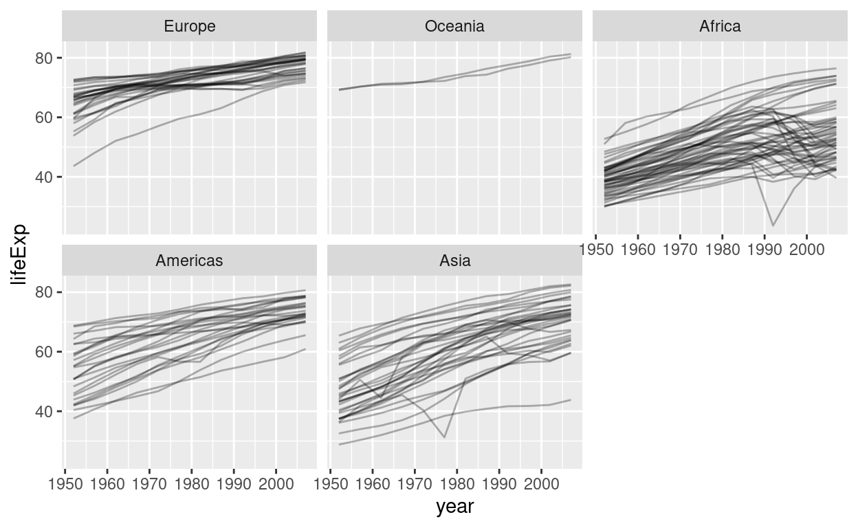
I saved the plot to a variable called plt because we need it later. Let’s make this plot a bit prettier by adding color! The gapminder package that provided this dataset also included a nice color palette. I included it as a .csv file in the data/ folder so that we can practice importing data once more. But you could also take the shortcut of getting it straight from the package (gapminder::country_colors). Here, we are using the head function to look at the first couple of rows of the tibble and to look at the first couple of elements of the named vector from the package.

country_colors <- read_csv("data/country_colors.csv")
head(country_colors)

# A tibble: 6 x 2
  country          color  
  <chr>            <chr>  
1 Nigeria          #7F3B08
2 Egypt            #833D07
3 Ethiopia         #873F07
4 Congo, Dem. Rep. #8B4107
5 South Africa     #8F4407
6 Sudan            #934607

head(gapminder::country_colors)

         Nigeria            Egypt         Ethiopia Congo, Dem. Rep. 
       "#7F3B08"        "#833D07"        "#873F07"        "#8B4107" 
    South Africa            Sudan 
       "#8F4407"        "#934607"

Notice, that the csv that we read in translates to a tibble with two columns, namely country and color. But what we need for ggplot to assign colors to the countries is what the gapminder package provides: a names vector. The names are the countries and the values so called hexadecimal (short Hex) color codes (https://www.w3schools.com/colors/colors_hexadecimal.asp). So what we want to do is translate the tibble into a named vector:

country_colors <- country_colors %>% 
  mutate(color = set_names(color, country)) %>% 
  pull(color)

head(country_colors)

         Nigeria            Egypt         Ethiopia Congo, Dem. Rep. 
       "#7F3B08"        "#833D07"        "#873F07"        "#8B4107" 
    South Africa            Sudan 
       "#8F4407"        "#934607"

Two things happened here that are sort of new. set_names is a handy way to take a vector and return a vector with names. It fits better into the tidyverse syntax than the “old” way of assigning to names(x) <- c("new", "names", "vector"). And secondly pull can be though of as a pipeable dollar. It pulls out the column of a tibble or the element of a named list.

gapminder$year %>% head()

[1] 1952 1957 1962 1967 1972 1977

gapminder %>% pull(year) %>% head()

[1] 1952 1957 1962 1967 1972 1977

Now, with our color vector ready to go, we can make the plot pretty. Remember the variable we saved our plot to? We can add more ggplot functions to it just like to a regular ggplot. A guide is the generalization of a legend, so we are setting it to none because adding a legend for 142 different colors (/countries) would fill the whole plot.

plt +
  aes(color = country) +
  scale_color_manual(values = country_colors, guide = guide_none()) +
  theme_minimal() + 
  labs(x = "",
       y = "Life Expectancy at Birth",
       title = "Life Expectancy over Time")

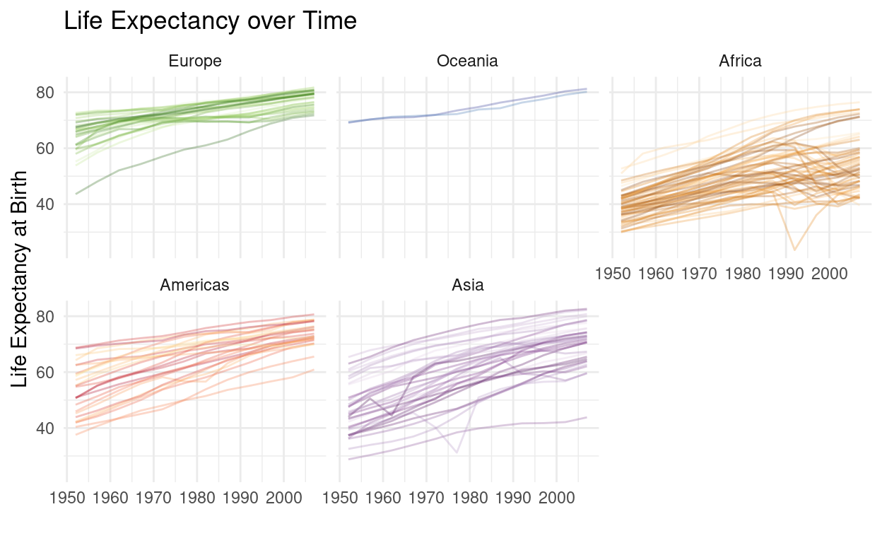
We also added a theme and modified the axis titles. You might have already notice a number of very pronounced dips in some of the lines. We will investigate this rather bleak reality when we talk about modeling and iteration next week.

Exercises

Drink a cup of coffee or tea, relax, because you just worked through quite a long video.
Familiarize yourself with the folders on your computer. Make sure you understand, where your directories and files live.
From RStudio, create a new RStudio project for this course.
- Inside the project folder, create a folder for the data.
- Create a new Rmarkdown document at the top level of your project folder for today’s exercises, again including questions that came up during the course.
- Download the data for today in one of the ways taught. You can refer to the script anytime.
- Make sure you have all the important settings set and are feeling right at home in RStudio.
The file ./data/exercise1.txt is in an unfamiliar format.
- Find out how it is structured and read it as a tibble.
- Create a scatterplot of the x and y column with ggplot2.
- Look at the help page for geom_point. What is the difference between geom_point(aes(color = <something>)) and geom_point(color = <something>)? A relevant hint is in the section about the ...-argument.
- Make the plot pretty by coloring the points, keeping in mind the above distinction.
Read in the gapminder dataset with readr
- Using a combination of dplyr verbs and / or visualizations with ggplot2, answer the following questions:
- Which continent had the highest life expectancy on average in the most current year? There are two options here. First, calculate a simple mean for the countries in each continent. Then, remember that the countries have different population sizes, so we really need a weighted mean using R’s function weighted.mean().
- Is there a relationship between the GDP per capita and the life expectancy? A visualization might be helpful.
- How did the population of the countries change over time? Make the plot more informative by adding color, facets and labels (with geom_text). Can you find out, how to add the country name label only to the last year? Hint: Have a look at the data argument that all geom_-functions have.

Resources

Package Documentation

Getting Help

“Artwork by @Allison_horst.” 2020. https://github.com/allisonhorst/stats-illustrations.

Bryan, Jennifer. 2017. Gapminder: Data from Gapminder. Manual.

Wickham, Hadley, and Garrett Grolemund. 2017. R for Data Science: Import, Tidy, Transform, Visualize, and Model Data. 1 edition. Sebastopol, CA: O’Reilly Media.

Lecture 2

Video

Slides

Script

Making Ourselves at Home in RStudio

Important Settings

A Project-based Workflow

Working in Style

A Data Analysis Workflow

Reading Data with `readr`

Common Hurdles when Importing Data

Wrangling Data with `dplyr`

select

filter

mutate

Interlude: Begind the magic, handling data with base-R

The pipe `%>%`

arrange

summarise

group_by

Visualization and our First Encounter with `factor`s

Exercises

Resources

Package Documentation

Getting Help

References

Corrections

Reuse

Citation

Lecture 2

Video

Slides

Script

Making Ourselves at Home in RStudio

Important Settings

A Project-based Workflow

Working in Style

A Data Analysis Workflow

Reading Data with readr

Common Hurdles when Importing Data

Wrangling Data with dplyr

select

filter

mutate

Interlude: Begind the magic, handling data with base-R

The pipe %>%

arrange

summarise

group_by

Visualization and our First Encounter with factors

Exercises

Resources

Package Documentation

Getting Help

References

Corrections

Reuse

Citation

Reading Data with `readr`

Wrangling Data with `dplyr`

The pipe `%>%`

Visualization and our First Encounter with `factor`s