3  Tidy data

… in which we explore the concept of Tidy Data and learn more advanced data wrangling techniques

Once again, we start by loading the tidyverse. In the lecture video you can also see a recap, a speed run of sorts, of lectures 1 and 2.

library(tidyverse)

3.1 Tidy data

Let’s get started with this pivotal topic.

3.1.1 What and why is tidy data?

There is one concept which also lends it’s name to the tidyverse that I want to talk about. Tidy Data is a way of turning your datasets into a uniform shape. This makes it easier to develop and work with tools because we get a consistent interface. Once you know how to turn any dataset into a tidy dataset, you are on home turf and can express your ideas more fluently in code. Getting there can sometimes be tricky, but I will give you the most important tools.

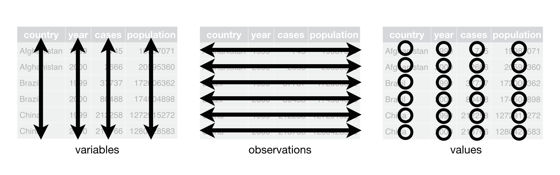
In tidy data, each variable (feature) forms it’s own column. Each observation forms a row. And each cell is a single value (measurement). Furthermore, information about the same things belongs in one table.

Figure from https://r4ds.had.co.nz/tidy-data.html Wickham and Grolemund (2017)

3.1.2 Make data tidy

with the tidyr package.

“Happy families are all alike; every unhappy family is unhappy in its own way”
— Leo Tolstoy (https://tidyr.tidyverse.org/articles/tidy-data.html)

And this quote holds true for messy datasets as well. The tidyr package contained in the tidyverse provides small example datasets to demonstrate what this means in practice. Hadley Wickham and Garrett Grolemund use these in their book as well (https://r4ds.had.co.nz/tidy-data.html)(Wickham and Grolemund 2017).

Let’s make some data tidy!

table1, table2, table3, table4a, table4b, and table5 all display the number of TB cases documented by the World Health Organization in Afghanistan, Brazil, and China between 1999 and 2000. The first of these is in the tidy format, the others are not:

table1

# A tibble: 6 × 4
  country      year  cases population
  <chr>       <dbl>  <dbl>      <dbl>
1 Afghanistan  1999    745   19987071
2 Afghanistan  2000   2666   20595360
3 Brazil       1999  37737  172006362
4 Brazil       2000  80488  174504898
5 China        1999 212258 1272915272
6 China        2000 213766 1280428583

This nicely qualifies as tidy data. Every row is uniquely identified by the country and year, and all other columns are properties of the specific country in this specific year.

3.1.3 pivot_wider

Now it gets interesting. table2 still looks organized, but it is not tidy (by our definition). Note, this doesn’t say the format is useless — it has it’s places — but it will not fit in as snugly with our tools. The column type is not a feature of the country, rather the actual features are hidden in that column with their values in the count column.

table2

# A tibble: 12 × 4
   country      year type            count
   <chr>       <dbl> <chr>           <dbl>
 1 Afghanistan  1999 cases             745
 2 Afghanistan  1999 population   19987071
 3 Afghanistan  2000 cases            2666
 4 Afghanistan  2000 population   20595360
 5 Brazil       1999 cases           37737
 6 Brazil       1999 population  172006362
 7 Brazil       2000 cases           80488
 8 Brazil       2000 population  174504898
 9 China        1999 cases          212258
10 China        1999 population 1272915272
11 China        2000 cases          213766
12 China        2000 population 1280428583

In order to make it tidy, this dataset would needs become wider.

table2 %>% 
  pivot_wider(names_from = type, values_from = count)

# A tibble: 6 × 4
  country      year  cases population
  <chr>       <dbl>  <dbl>      <dbl>
1 Afghanistan  1999    745   19987071
2 Afghanistan  2000   2666   20595360
3 Brazil       1999  37737  172006362
4 Brazil       2000  80488  174504898
5 China        1999 212258 1272915272
6 China        2000 213766 1280428583

3.1.4 separate

In table3, two features are jammed into one column. This is annoying, because we can’t easily calculate with the values; they are stored as text and separated by a slash like cases/population.

table3

# A tibble: 6 × 3
  country      year rate             
  <chr>       <dbl> <chr>            
1 Afghanistan  1999 745/19987071     
2 Afghanistan  2000 2666/20595360    
3 Brazil       1999 37737/172006362  
4 Brazil       2000 80488/174504898  
5 China        1999 212258/1272915272
6 China        2000 213766/1280428583

Ideally, we would want to separate this column into two:

table3 %>% 
  separate(col = rate, into = c("cases", "population"), sep = "/")

# A tibble: 6 × 4
  country      year cases  population
  <chr>       <dbl> <chr>  <chr>     
1 Afghanistan  1999 745    19987071  
2 Afghanistan  2000 2666   20595360  
3 Brazil       1999 37737  172006362 
4 Brazil       2000 80488  174504898 
5 China        1999 212258 1272915272
6 China        2000 213766 1280428583

3.1.5 pivot_longer

table4a and table4b split the data into two different tables, which again makes it harder to calculate with. This data is so closely related, we would want it in one table. And another principle of tidy data is violated. Notice the column names? 1999 is not a feature that Afghanistan can have. Rather, it is the value for a feature (namely the year), while the values in the 1999 column are in fact values for the feature population (in table4a) and cases (in table4b).

table4a

# A tibble: 3 × 3
  country     `1999` `2000`
  <chr>        <dbl>  <dbl>
1 Afghanistan    745   2666
2 Brazil       37737  80488
3 China       212258 213766

table4b

# A tibble: 3 × 3
  country         `1999`     `2000`
  <chr>            <dbl>      <dbl>
1 Afghanistan   19987071   20595360
2 Brazil       172006362  174504898
3 China       1272915272 1280428583

table4a %>% 
  pivot_longer(-country, names_to = "year", values_to = "cases")

# A tibble: 6 × 3
  country     year   cases
  <chr>       <chr>  <dbl>
1 Afghanistan 1999     745
2 Afghanistan 2000    2666
3 Brazil      1999   37737
4 Brazil      2000   80488
5 China       1999  212258
6 China       2000  213766

table4b %>% 
  pivot_longer(-country, names_to = "year", values_to = "population")

# A tibble: 6 × 3
  country     year  population
  <chr>       <chr>      <dbl>
1 Afghanistan 1999    19987071
2 Afghanistan 2000    20595360
3 Brazil      1999   172006362
4 Brazil      2000   174504898
5 China       1999  1272915272
6 China       2000  1280428583

We have another case where we are doing a very similar thing twice. There is a general rule of thumb that says:

“If you copy and paste the same code 3 times, you should probably write a function.”

This no only has the advantage of reducing code duplication and enabling us to potentially reuse our code later in another project, it also aids readability because we are forced to give this stop a name.

clean_wide_data <- function(data, values_column) {
  data %>% 
    pivot_longer(-country, names_to = "year", values_to = values_column)
}

We can then use this function for both tables.

clean4a <- table4a %>% 
  clean_wide_data("cases")

clean4b <- table4b %>% 
  clean_wide_data("population")

3.1.6 left_join

Now is the time to join clean4a and clean4b together. For this, we need an operation known from databases as a join. In fact, this whole concept of tidy data is closely related to databases and something called Codd`s normal forms (Codd 1990; Wickham 2014) so I am throwing these references in here just in case you are interested in the theoretical foundations. But without further ado:

left_join(clean4a, clean4b, by = c("country", "year"))

# A tibble: 6 × 4
  country     year   cases population
  <chr>       <chr>  <dbl>      <dbl>
1 Afghanistan 1999     745   19987071
2 Afghanistan 2000    2666   20595360
3 Brazil      1999   37737  172006362
4 Brazil      2000   80488  174504898
5 China       1999  212258 1272915272
6 China       2000  213766 1280428583

3.1.7 unite

In table5, we have the same problem as in table3 and additionally the opposite problem! This time, feature that should be one column (namely year) is spread across two columns (century and year).

table5

# A tibble: 6 × 4
  country     century year  rate             
  <chr>       <chr>   <chr> <chr>            
1 Afghanistan 19      99    745/19987071     
2 Afghanistan 20      00    2666/20595360    
3 Brazil      19      99    37737/172006362  
4 Brazil      20      00    80488/174504898  
5 China       19      99    212258/1272915272
6 China       20      00    213766/1280428583

What we want to do is unite those into one, and also deal with the other problem. However, we when do this we find out the our newly created year, cases and population columns are actually stored as text, not numbers! So in the next step, we convert those into numbers with the parse_number function.

table5 %>% 
  unite("year", century, year, sep = "") %>% 
  separate(rate, c("cases", "population")) %>% 
  mutate(
    year = parse_number(year),
    cases = parse_number(cases),
    population = parse_number(population)
  )

# A tibble: 6 × 4
  country      year  cases population
  <chr>       <dbl>  <dbl>      <dbl>
1 Afghanistan  1999    745   19987071
2 Afghanistan  2000   2666   20595360
3 Brazil       1999  37737  172006362
4 Brazil       2000  80488  174504898
5 China        1999 212258 1272915272
6 China        2000 213766 1280428583

parse_number is a bit like a less strict version of as.numeric. While as.numeric can only deal with text that contains only a number and nothing else, parse_number can help us by extracting numbers even if there is some non-number text around them:

as.numeric("we have 42 sheep")

[1] NA

parse_number handles this, no questions asked:

parse_number("we have 42 sheep")

[1] 42

Notice, how we applied the same function parse_number to multiple columns of our data? If we notice such a pattern, where there is lot’s of code repetition, chances are that there is a more elegant solution. You don’t have to find that elegant solution at first try, but keeping an open mind will improve your code in the long run. In this case, let me tell you about the across function. We can use it inside of dplyr verbs such as mutate and summarise to apply a function to multiple columns:

table5 %>% 
  unite("year", century, year, sep = "") %>% 
  separate(rate, c("cases", "population")) %>% 
  mutate(
    across(c(year, cases, population), parse_number)
  )

# A tibble: 6 × 4
  country      year  cases population
  <chr>       <dbl>  <dbl>      <dbl>
1 Afghanistan  1999    745   19987071
2 Afghanistan  2000   2666   20595360
3 Brazil       1999  37737  172006362
4 Brazil       2000  80488  174504898
5 China        1999 212258 1272915272
6 China        2000 213766 1280428583

As it’s first argument it takes a vector of column names (the c(...) bit) or a tidy-select specification (see ?dplyr_tidy_select) and as it’s second argument either one function or even a list of functions (with names).

Another way of specifying what columns to use here would be to say “every column but the country” with -country.

table5 %>% 
  unite("year", century, year, sep = "") %>% 
  separate(rate, c("cases", "population")) %>% 
  mutate(
    across(-country, parse_number)
  )

# A tibble: 6 × 4
  country      year  cases population
  <chr>       <dbl>  <dbl>      <dbl>
1 Afghanistan  1999    745   19987071
2 Afghanistan  2000   2666   20595360
3 Brazil       1999  37737  172006362
4 Brazil       2000  80488  174504898
5 China        1999 212258 1272915272
6 China        2000 213766 1280428583

3.1.8 Another example

Let us look at one last example of data that needs tidying, which is also provided by the tidyr package as an example:

head(billboard)

# A tibble: 6 × 79
  artist      track date.entered   wk1   wk2   wk3   wk4   wk5   wk6   wk7   wk8
  <chr>       <chr> <date>       <dbl> <dbl> <dbl> <dbl> <dbl> <dbl> <dbl> <dbl>
1 2 Pac       Baby… 2000-02-26      87    82    72    77    87    94    99    NA
2 2Ge+her     The … 2000-09-02      91    87    92    NA    NA    NA    NA    NA
3 3 Doors Do… Kryp… 2000-04-08      81    70    68    67    66    57    54    53
4 3 Doors Do… Loser 2000-10-21      76    76    72    69    67    65    55    59
5 504 Boyz    Wobb… 2000-04-15      57    34    25    17    17    31    36    49
6 98^0        Give… 2000-08-19      51    39    34    26    26    19     2     2
# ℹ 68 more variables: wk9 <dbl>, wk10 <dbl>, wk11 <dbl>, wk12 <dbl>,
#   wk13 <dbl>, wk14 <dbl>, wk15 <dbl>, wk16 <dbl>, wk17 <dbl>, wk18 <dbl>,
#   wk19 <dbl>, wk20 <dbl>, wk21 <dbl>, wk22 <dbl>, wk23 <dbl>, wk24 <dbl>,
#   wk25 <dbl>, wk26 <dbl>, wk27 <dbl>, wk28 <dbl>, wk29 <dbl>, wk30 <dbl>,
#   wk31 <dbl>, wk32 <dbl>, wk33 <dbl>, wk34 <dbl>, wk35 <dbl>, wk36 <dbl>,
#   wk37 <dbl>, wk38 <dbl>, wk39 <dbl>, wk40 <dbl>, wk41 <dbl>, wk42 <dbl>,
#   wk43 <dbl>, wk44 <dbl>, wk45 <dbl>, wk46 <dbl>, wk47 <dbl>, wk48 <dbl>, …

This is a lot of columns! For 76 weeks after a song entered the top 100 (I assume in the USA) its position is recorded. It might be in this format because it made data entry easier, or the previous person wanted to make plots in excel, where this wide format is used to denote multiple traces. In any event, for our style of visualizations with the grammar of graphics, we want a column to represent a feature, so this data needs to get longer:

billboard %>% 
  pivot_longer(starts_with("wk"), names_to = "week", values_to = "placement") %>% 
  mutate(week = parse_number(week)) %>% 
  head()

# A tibble: 6 × 5
  artist track                   date.entered  week placement
  <chr>  <chr>                   <date>       <dbl>     <dbl>
1 2 Pac  Baby Don't Cry (Keep... 2000-02-26       1        87
2 2 Pac  Baby Don't Cry (Keep... 2000-02-26       2        82
3 2 Pac  Baby Don't Cry (Keep... 2000-02-26       3        72
4 2 Pac  Baby Don't Cry (Keep... 2000-02-26       4        77
5 2 Pac  Baby Don't Cry (Keep... 2000-02-26       5        87
6 2 Pac  Baby Don't Cry (Keep... 2000-02-26       6        94

Let’s save this to a variable. And while we are at it, we can save the extra mutate-step by performing the transformation from text to numbers right inside of the pivot_longer function.

tidy_bilboard <- billboard %>% 
  pivot_longer(starts_with("wk"),
    names_to = "week",
    values_to = "placement",
    names_prefix = "wk",
    names_transform = list(week = as.integer)
  )

tidy_bilboard %>% head(10)

# A tibble: 10 × 5
   artist track                   date.entered  week placement
   <chr>  <chr>                   <date>       <int>     <dbl>
 1 2 Pac  Baby Don't Cry (Keep... 2000-02-26       1        87
 2 2 Pac  Baby Don't Cry (Keep... 2000-02-26       2        82
 3 2 Pac  Baby Don't Cry (Keep... 2000-02-26       3        72
 4 2 Pac  Baby Don't Cry (Keep... 2000-02-26       4        77
 5 2 Pac  Baby Don't Cry (Keep... 2000-02-26       5        87
 6 2 Pac  Baby Don't Cry (Keep... 2000-02-26       6        94
 7 2 Pac  Baby Don't Cry (Keep... 2000-02-26       7        99
 8 2 Pac  Baby Don't Cry (Keep... 2000-02-26       8        NA
 9 2 Pac  Baby Don't Cry (Keep... 2000-02-26       9        NA
10 2 Pac  Baby Don't Cry (Keep... 2000-02-26      10        NA

Yes, those pivot functions are really powerful!

A notable difference that often happens between long- and wide-format data is the way missing data is handled.

Because every row needs to have the same number of columns, and in the wide format every column is a week, there are bound to be a lot of NA values wherever a song was simply no longer in the top 100 at the specified week. Those missing values are then very explicit.

In the long format we have the option to make the missing values implicit by simply omitting the row where there is no meaningful information. With the function na.omitt for example, we can remove all rows that have NA somewhere:

tidy_bilboard %>%
  head(10) %>% 
  na.omit()

# A tibble: 7 × 5
  artist track                   date.entered  week placement
  <chr>  <chr>                   <date>       <int>     <dbl>
1 2 Pac  Baby Don't Cry (Keep... 2000-02-26       1        87
2 2 Pac  Baby Don't Cry (Keep... 2000-02-26       2        82
3 2 Pac  Baby Don't Cry (Keep... 2000-02-26       3        72
4 2 Pac  Baby Don't Cry (Keep... 2000-02-26       4        77
5 2 Pac  Baby Don't Cry (Keep... 2000-02-26       5        87
6 2 Pac  Baby Don't Cry (Keep... 2000-02-26       6        94
7 2 Pac  Baby Don't Cry (Keep... 2000-02-26       7        99

Let’s reward ourselves with a little visualization. Here, I am also introducing the plotly package, which has the handy function ggplotly to turn a regular ggplot into an interactive plot. Plotly also has its own way of building plots, which you might want to check out for advanced interactive or 3-dimensional plots: https://plotly.com/r/, but for the most part we don’t need to worry about it due to the amazingly simple ggplotly translation function.

plt <- tidy_bilboard %>% 
  ggplot(aes(week, placement)) +
  geom_point(aes(label = paste(artist, track))) +
  geom_line(aes(group = paste(artist, track)))

plotly::ggplotly(plt)

This whole tidy data idea might seem like just another way of moving numbers around. But once you build the mental model for it, it will truly transform the way you are able to think about data. Both for data wrangling with dplyr, as shown last week, and also for data visualization with ggplot, a journey we began in the first week and that is still well underway.

3.2 More shapes for data

Data comes in many shapes and R has more than just vectors and dataframes / tibbles. I this course we are omitting matrices, which store data of the same type in 2 dimensions, and it’s multi-dimensional equivalent arrays.

What we are not omitting, and in fact have already teased but never properly defined is lists.

3.2.1 Lists

On first glance, lists are very similar to atomic vectors, as they are both one dimensional data structures and both of them can have names.

c(first = 1, second = 2)

 first second 
     1      2 

list(first = 1, second = 2)

$first
[1] 1

$second
[1] 2

What sets them apart is that while atomic vectors can only contain data of the same type (like only numbers or only text), a list can contain anything, even other lists!

x <- list(first = 1, second = 2, "some text", list(1, 2), 1:5)
x

$first
[1] 1

$second
[1] 2

[[3]]
[1] "some text"

[[4]]
[[4]][[1]]
[1] 1

[[4]][[2]]
[1] 2


[[5]]
[1] 1 2 3 4 5

As it turns out, dataframes internally are also lists, namely a list of columns. They just have some more properties (which R calls attributes) that tell R to display it in the familiar rectangular shape.

palmerpenguins::penguins %>% head()

# A tibble: 6 × 8
  species island    bill_length_mm bill_depth_mm flipper_length_mm body_mass_g
  <fct>   <fct>              <dbl>         <dbl>             <int>       <int>
1 Adelie  Torgersen           39.1          18.7               181        3750
2 Adelie  Torgersen           39.5          17.4               186        3800
3 Adelie  Torgersen           40.3          18                 195        3250
4 Adelie  Torgersen           NA            NA                  NA          NA
5 Adelie  Torgersen           36.7          19.3               193        3450
6 Adelie  Torgersen           39.3          20.6               190        3650
# ℹ 2 more variables: sex <fct>, year <int>

3.2.2 Nested data

The tidyr package provides more tools for dealing with data in various shapes. We just discovered the first set of operations called pivots and joins to get a feel for tidy data and to obtain it from various formats. But data is not always rectangular like we can show it in a spreadsheet. Sometimes data already comes in a nested form, sometimes we create nested data because it serves our purpose. So, what do I mean by nested?

Remember that lists can contain elements of any type, even other lists. If we have a list that contains more lists, we call it nested e.g.

list(
  c(1, 2),
  list(
    42, list("hi", TRUE)
  )
)

But nested list are not always fun to work with, and when there is a straightforward way to represent the same data in a rectangular, flat format, we most likely want to do that. We will deal with data rectangling today was well. But first, there is another implication of nested lists:

Because dataframes (and tibbles) are built on top of lists, we can nest them to! This can sometimes come in really handy. We a dataframe contains a column that is not an atomic vector but a list (so it is a list in a list), we call it a list column:

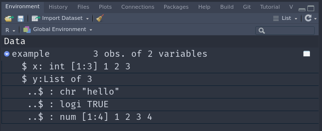
example <- tibble(
  x = 1:3,
  y = list(
    "hello",
    TRUE,
    1:4
  )
)

example

# A tibble: 3 × 2
      x y        
  <int> <list>   
1     1 <chr [1]>
2     2 <lgl [1]>
3     3 <int [4]>

# View(example)

Use the View function, or the click in the environment panel to inspect the nested data with a better overview.

Of course we are unlikely to build these nested tibbles by hand with the tibble function. Instead, our data usually comes from some dataset we are working with. Let’s take the familiar penguins dataset and nest it.

nested <- palmerpenguins::penguins %>% 
  nest(data = -island)

nested

# A tibble: 3 × 2
  island    data              
  <fct>     <list>            
1 Torgersen <tibble [52 × 7]> 
2 Biscoe    <tibble [168 × 7]>
3 Dream     <tibble [124 × 7]>

nest has a syntax similar to mutate, where we first specify the name of the column to create (we call it data here), followed by a specification of the columns to nest into that list column.

Our data column is now a list of tibbles and each individual tibble in the list contains the data for the species of that row. Looking into the data column’s first element, we can see that it is indeed a regular tibble and didn’t take it personal to get stuffed into a list column.

nested$data[[1]]

# A tibble: 52 × 7
   species bill_length_mm bill_depth_mm flipper_length_mm body_mass_g sex   
   <fct>            <dbl>         <dbl>             <int>       <int> <fct> 
 1 Adelie            39.1          18.7               181        3750 male  
 2 Adelie            39.5          17.4               186        3800 female
 3 Adelie            40.3          18                 195        3250 female
 4 Adelie            NA            NA                  NA          NA <NA>  
 5 Adelie            36.7          19.3               193        3450 female
 6 Adelie            39.3          20.6               190        3650 male  
 7 Adelie            38.9          17.8               181        3625 female
 8 Adelie            39.2          19.6               195        4675 male  
 9 Adelie            34.1          18.1               193        3475 <NA>  
10 Adelie            42            20.2               190        4250 <NA>  
# ℹ 42 more rows
# ℹ 1 more variable: year <int>

To unnest the column again we use the function unnest. Sometimes we need to be specific and use unnest_wider or unnest_longer, but here the automatic unnest makes the right choices already.

nested %>% 
  unnest(data)

# A tibble: 344 × 8
   island    species bill_length_mm bill_depth_mm flipper_length_mm body_mass_g
   <fct>     <fct>            <dbl>         <dbl>             <int>       <int>
 1 Torgersen Adelie            39.1          18.7               181        3750
 2 Torgersen Adelie            39.5          17.4               186        3800
 3 Torgersen Adelie            40.3          18                 195        3250
 4 Torgersen Adelie            NA            NA                  NA          NA
 5 Torgersen Adelie            36.7          19.3               193        3450
 6 Torgersen Adelie            39.3          20.6               190        3650
 7 Torgersen Adelie            38.9          17.8               181        3625
 8 Torgersen Adelie            39.2          19.6               195        4675
 9 Torgersen Adelie            34.1          18.1               193        3475
10 Torgersen Adelie            42            20.2               190        4250
# ℹ 334 more rows
# ℹ 2 more variables: sex <fct>, year <int>

3.3 Exercises

3.3.1 Tidy data

For the first set of exercises I am cheating a little and take those from the (absolutely brilliant) book R for Data Science (Wickham and Grolemund 2017) by the original creator of much of the tidyverse. So, for the first part, solve / answer the 4 questions found here: https://r4ds.had.co.nz/tidy-data.html#exercises-24

I do have to give another hint, because I haven’t mentioned it so far: When I introduced variables I told you that those can only contain letters, underscores and numbers and are not allowed to start with a number. However, we can use “illegal” names for variables and columns if the surround them with backticks, e.g.:

`illegal variable` <- 42
`illegal variable`

[1] 42

This is how Hadley can refer to the columns named after years in pivot_longer in exercise 1.

3.3.2 A new dataset: airlines

• Imagine for a second this whole pandemic thing is not going on and we are planning a vacation. Of course, we want to choose the safest airline possible. So we download data about incident reports. You can find it in the ./data/03/ folder.
• Instead of the type_of_event and n_events columns we would like to have one column per type of event, where the values are the count for this event.
• Which airlines had the least fatal accidents? What happens if we standardized these numbers to the distance theses airlines covered in the two time ranges?
• Which airlines have the best record when it comes to fatalities per fatal accident?
• Create informative visualizations and / or tables to communicate your discoveries. It might be beneficial to only plot e.g. the highest or lowest scoring Airlines. One of the slice_ functions will help you there. And to make your plot more organized, you might want to have a look into fct_reorder.

3.4 Resources

• tidyr documentation
• purrr documentation
• stringr documentation for working with text and a helpful cheatsheet for the regular expressions mentioned in the video

Codd, E. F. 1990. The Relational Model for Database Management: Version 2. USA: Addison-Wesley Longman Publishing Co., Inc.

Wickham, Hadley. 2014. “Tidy Data.” Journal of Statistical Software 59 (1): 1–23. https://doi.org/10.18637/jss.v059.i10.

Wickham, Hadley, and Garrett Grolemund. 2017. R for Data Science: Import, Tidy, Transform, Visualize, and Model Data. 1 edition. Sebastopol, CA: O’Reilly Media.